• ExampleBC -- a box that is 20 units x 20 units with 0V around all the edges except the bottom; the bottom side of the box has a voltage of 100V.

• ParallelPlateBC -- a parallel-plate transmission line with the bottom plate at a voltage of -100V and the top plate at a voltage of +100V.

• TwoLineBC -- a two-wire transmission line with the bottom line at a voltage of -100V and the top line at a voltage of +100V.

• CoaxialBC -- a coaxial transmission line with the outer conductor at 0V and the inner conductor at 100V.

• MicrostripBC -- a microstrip transmission line with the ground plane at 0V and the upper strip line at 100V.

Syntax:  V = PlotVoltageXY( BoundaryConditions, EquipotentialLines, MaximumIterations, Tolerance )

Example:  V = PlotVoltageXY(ExampleBC,[100 50 30 20 10 5 2 1 0]);

Inputs:

• BoundaryConditions -- The boundary condition matrix can be any dimension NxM. If a location in the matrix represents a boundary condition, simply set that point equal to the boundary voltage. If voltage at a location is to be calculated, set that equal to the NaN value. For this type of relaxation algorithm, the boundary conditions around the edge of the matrix must be specified. Other points in the boundary condition matrix are optional.

• EquipotentialLines -- An array of voltage values for equipotential lines to plot in the final figure.

• MaximumIterations (optional) -- Number of iterations in the relaxation calculation.

• Tolerance (optional) -- Threshold change between iterations that detects convergence; the stopping criterion.

Outputs:

• V -- The final voltage matrix

• Plots of the voltage map and equipotential lines.

Notes:

• This code was developed and tested on Release 13 of Matlab^TM.  It may require a few alterations to run on earlier releases.

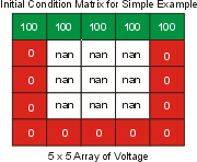
• The boundary conditions matrix for the 5 x 5 example calculation could be constructed with the following lines of code:
  >> BC = repmat(nan,5,5);
  >> BC(:,1) = 0;
  >> BC(:,end) = 0;
  >> BC(1,:) = 0;
  >> BC(end,:) = 100;
  >> BC
  
  BC =
  
  0   0   0   0   0
  0   NaN NaN NaN 0
  0   NaN NaN NaN 0
  0   NaN NaN NaN 0
  100 100 100 100 100
  
  The resulting boundary conditions are shown below (note the vertically flipped conventions since Matlab numbers its matrix rows from top to bottom with increasing indices, whereas our coordinate system requires y to be increasing from bottom to top):

• If you would like to see the individual iterations displayed in a window during the relaxation calculation, change the first line of code to FAST=false;. This will enable a colorful animation that shows the computation of the voltages in space.  The drawback is that the animation slows down the overall calculation substantially.