The Shinkansen (Japanese bullet train) provides a harsh radio propagation environment for cellular phones. In order for NTT DoCoMo to provide quality and reliable cellular service inside a train, a sophisticated receiver structure must be deployed. Using two monopole antennas placed 2 meters apart with a selection diversity system should improved the receiving signal of the mobile repeater greatly.  However, the switching speed between the two antennas can only be determined with proper simulation of the receiving signal strength of both antennas.

 

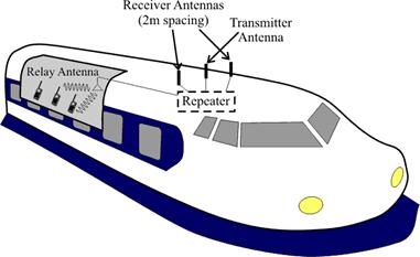
Figure 1:  Diagram of the bullet train repeater with diversity antennas

 

            The bullet train will travel in two types of environment. One is the open rural area with little multipath interference. In this case the angle spectrum of the antenna pattern will be set to 3 degrees width. The second environment is the urban area with high multipath interference. For this case we will set the angle spectrum of the antenna pattern to 120 degrees width. We will analyze the receiving signal strength when the train is traveling towards the base station and transverse to the base station.

 

            In order to simulate the receiving signal strength with certain multipath azimuth spectra, we have to find the total electric field in the z direction from incoming radio waves arriving from all directions. Since the antennas are pointing in the z direction, only the z component of the radio wave can excite a received signal.

 

            We can simulate the z component of many radio waves coming from all direction with random phases with the following equation:

 

 

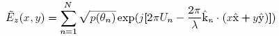
This equation was implemented in MATLAB to determine the signal strength of the antenna that is laying on the x axis. Since the train is always traveling in the x direction, we can remove the y component in the equation.  The second antenna is placed 2 meters below the first, on the y axis. We must create another vector of electric fields in the z direction using the above equation with y equals to -2 meters.

Figure 2:  Antenna placement

 

 

The first case we will analyze is the rural environment with the train traveling towards and transverse to the base station. (Double click on figure 3 or figure 4 to see the signal strength change as the train moves forward)

 

Figure 3:  Train traveling in the direction of base station with 3 degree angle spectrum

Figure 4:  Train traveling transverse to direction of the base station with 3 degree angle spectrum

 

 

            In Figure 3 the train is traveling towards the base station. The signal strength of both antennas does not fluctuate much as when the train is traveling transversely. This is because the distance between antenna 1 to the base station is almost the same as antenna 2 to the base station. And since both antennas are traveling towards the base station at the same speed, the incoming radio wave they receive is more or less the same.

 

            In Figure 4 the train is traveling transversely to the base station. This means the antennas are place at an angle of maximum fading, which causes the signal to fade more often then the signal in Figure 3. The periodicity of the signal strength is due the high directional gain of the antenna pattern when the angle spectrum is at 3 degrees. And since the antennas can only see small amount of incoming waves, the sum of these propagating waves will seem periodic.

 

The second case we will analyze is the urban environment with the train traveling towards and transverse to the base station. Due high amount of multipath interference we will change the width angle spectrum to 120 degrees width.  (Double click on figure 5 or figure 6 to see the signal strength change as the train moves forward)

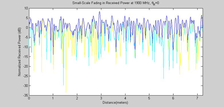
Figure 5:  Train traveling in the direction of the base station with 120 degree angle spectrum

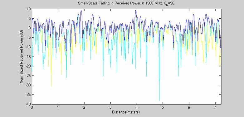
Figure 6: Train traveling transverse to the direction of the base station with 120 degree angle spectrum

            In a high multipath environment with antennas having a wide angle spectrum will allow the antennas to receive a large number of incoming waves from all direction. This causes much larger fluctuation in signal strength then in rural areas. The average fade duration is going to decrease and the level crossing rate will increase.

 

 

Analytical calculations of level crossing rates and fade durations at speed of 260km/hr

 

The level crossing rate gives a good understanding of how fast the signal fluctuates at a giving threshold value.  The average fade duration describes the average time a signal spends under a threshold value.  These two values can help us in determining the speed we should switch between the two antennas.  The analytical equations for calculating the two values are

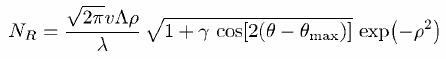
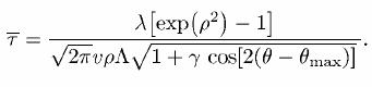
            These two equations were implemented in MATLAB with the train traveling towards and transverse to the base station with wide and narrow angle spectrum.

 

 

Figure 7: Level crossing rate

 

Figure 8:  Average fade duration

           

            Looking at Figure 7 we can see the maximum level crossing per second can be almost as high as 500 crossings per second. The level crossing rate of the signal that is being analyzed is made from a single antenna, therefore when switching between the two antennas we must do so twice as fast. By Shannon’s theorem we should sample the two antennas at least 2000 times per second.

 

Building a mobile repeater inside the bullet train with two diversity antenna placed two meters apart on top of the train can greatly increase the reliability of the signal strength inside the train.  Switching and sampling the two antennas at 2000 times per second will definitely give DoCoMo a marketing advantage over its chief rival, J-phone.