|
ECE 3065 Spring 2005 Project Finding the Power: A Study in Antenna Propagation The Problem: The largest North American cellular carrier, Springularizon, has deemed conventional propagation models outdated and obsolete. They desire to cost effectively position their cellular base stations in a way that would ensure the outstanding coverage for which they are so well known. Customer habits are changing and it is necessary that the cellular networks adapt to this change. If there is not enough coverage in any area that customers need it, they will leave and go to the outstanding cellular network of V02daxtel, costing Springularizon billions in lost revenue. Overcompensating will result in spending billions on unnecessary infrastructure. Either way it would mean fewer mansions and fewer trips on the private jets for the shareholders. It is therefore necessary that a state of the art propagation modeling software be developed to ideally determine the coverage a cellular base station provides in a given environment. There have been many books written on the theory of antenna propagation. They utilize a combination of Maxwell’s equations and Helmholtz free space wave equations to determine what shape the propagation pattern of an antenna is going to be. The link budget equation is also used to determine what power an antenna can be expected to receive from a given transmitter. However, things that look good on paper, especially in the area of RF get turned upside down and often look nothing like one would expect once implemented in the real world. The environment in which an antenna is deployed severely affects the actual signal that a receiver is going to receive. This is the basis for this investigation. Detailed data of the received signal strength from a total of eight cell phone towers around campus was gathered by Springularizon. The properties of each tower were given to the designer. This data was presented to the designer in the form of a Matlab struct file, which could then be further utilized and manipulated. It was the task of the designer to create a Matlab program that would as accurately as possible predict what powers would be received in any 10m x 10m area across campus from any of the eight towers that were measured. The Model: The model that was employed was developed in stages. This section will describe the stages that were gone through to get to the model that was submitted. The basis for calculating powers received across campus is the link budget equation, which is as follows: PR = PT + GT + GR + 20 log10(lambda / 4 pi) – 10 n log10(d / 1m) – APL Where PR is the power received, PT the power transmitted by the base station, GT the gain of the transmitter, GR the gain of the receiver, n is the propagation loss coeffictient, d is the distance to the transmitter, and APL is the Aggregate Penetration Loss. All the values in this equation are in dB. Problems with the models and areas of desired improvement will be discussed also at the end of this section.
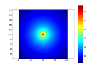
As a beginning for creating a propagation pattern for the different cellular base stations, a propagation canvas was created. The problem was designed such that the center of every propagation map was the location of the antenna. The program began by simply cycling through every square of the matrix which represented a location on campus, and calculating the power received using the link budget equation given above. However, a reduction factor was put in front of the gain due to the directive nature of the antennas. As a result of this step, the omni-directional pattern shown in Fig. 1 was produced.
Antenna Directivity: Since the antennas that are used in cellular base stations are directional, it was essential to be able to have an element of this in the propagation pattern. An antenna with a gain of 0 dB would be a perfect sphere. As the gain of an antenna increases, this simply indicates that power is being taken from one possible direction of propagation in that sphere and added to another.
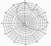
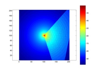
It was taken that a cellular base station antenna has a half power beam width of approximately 120o. Figure 2 roughly shows the propagation pattern of such an antenna. This roughly means that at the edges of a 120o angle looking away from the antenna, the antenna is transmitting half of its power in that direction. In the case of a directional antenna, such as this one, were one to stand in front of the antenna, the power received would be much greater than that of someone standing behind of the antenna. One of the properties that were given was the azimuth direction in which the antenna was pointed. The link budget equation was calculated inside general a 120o triangle. This was then rotated to the azimuth direction for the individual base station. The plane pattern values in these locations were replaced with this triangle. The product of this phase is shown below in figure 3.
Buildings: As was mentioned earlier in the report, the environment in which an antenna is operating severely affects the propagation pattern. One of the main focuses of this investigation was to try to model the effects being in a building would have on the power received from an antenna. This is were the n factor in the link budget equation comes into play. n is the propagation loss coefficient which can be calculated in for different environments and applied to the link budget equation in order to minimize the standard deviation between purely theoretical path loss calculations and actual readings in different environments. A value of 2 represents free space. High values represent different environments depending on the physical density or other properties of obstacles in the propagation medium.
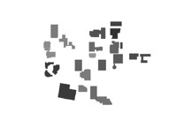
A grayscale image of the buildings on campus in which measurements where taken was provided. (Fig.4) This images was converted such that the size of the buildings matched 10m x 10m block of which the propagation maps were made. It was integrated into propagation map by shifting it such that the antenna was placed correctly between the buildings. The link budget equation was then changed so that when a block was at a point that corresponded to a building, the propagation loss coefficient was changed to a higher value.
As was mentioned earlier, an n value of 2 represented free space. However, given the density of the buildings on campus, a value of 3 was chosen for the outdoors and a value of 4 was used for the indoor blocks. This stage would have resulted in the final propagation pattern for this model as see in figure 5. Learning Algorithm: As a result of the difficulties involved in matching the size of the building mask shown in the previous section, it was desired to devise a way of better judging where the buildings were, and more so where the points where to which these predictions would be compared. What better tool than the maps of the measurements of the first four base stations that were provided? Contemplation was then done as to whether readings taken from one or more antennas in a particular environment could aid in predicting how other antennas placed in that environment would work. Namely, could the program “learn” from these measurements? A program was written that would make the plane theoretical predictions with directivity for the first four cells, subtract the difference of the actual measured data from these predictions and store them in a matrix. Since the matrices were done so that the antennas were always at the middle, each map was then shifted so that they would line up with their physical locations relative to the first cell. The shifted matrices were then added and averaged. In essence an aggregate propagation loss (APL) was created for each cell. Although there is some obvious unfairness with now comparing the standard deviations on the first four cells to the actual measurements, since properties of the actual measurements were used to predict those same measurements, the real interest lies in the outcome of the comparison to the four mystery cells. Will this attempt at “learning” about the environment with measurements from the first four cells aid in making predictions of the other four in the same environment?
Problems: There was some difficulty in aligning the building mask correctly to the antenna locations. This was done by guessing on what building one of the antennas was located and referencing it to a pixel on the mask. Shift was calculated from a the corresponding length of a degree of longitude and latitude around –84 lon, 33 lat. This could have been done more accurately.Improvements: As of now, the learning algorithm is simply averaging the difference between the measured data and the theoretical prediction. Having data from the four towers would better allow one to calculate a propagation loss coefficient for the different cells.
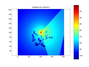
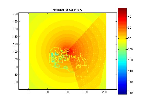
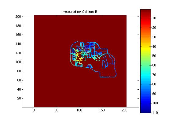
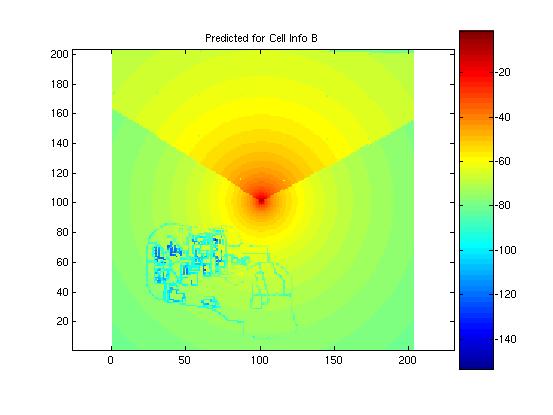
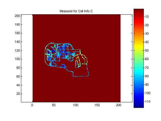
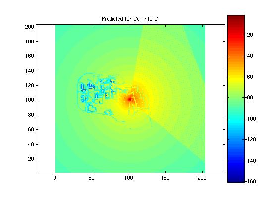
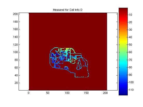
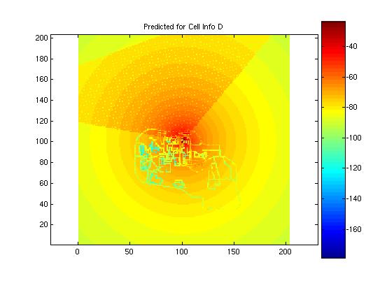
Actual measured data four the first four of the eight coverage maps were provided to the designer in order to test the performance of the models against actual data. Here the error of the shifting algorithm becomes evident. Were the learning matrices correctly positioned, it is believed that the mean error and standard deviation would have been much less. Here the actual measured data for the first four cells is presented and compared to the predicted model. The mean and standard deviation for the model is presented in the figure with the predicted propagation pattern. It is evident in these images that there was a problem with the shifting algorithm. The antenna locations appear clos for some of the predictions, as is the case in cell A, but way of for other location, as in cell B. Nonetheless, the addition of the learning matrix did tend to improve the standard deviation of the predictions by several dB.
Cell B:
Cell C:
Cell D:
Application to a nation-wide cellular network. The object of developing this propagation modeling software for Springularizon was to be able to apply it to their nationwide network. There are a couple problems which are evident when considering such a program on this scale. Without considering the learning algorithm, calculating the propagation map just for the Georgia Tech campus takes almost minutes. This was just a 203x203 block of 10m x 10m squares that was being computed. If one would consider the metro Atlanta area alone, Springularizon would have to spend the money that would go to extra infrastructure simply on the computing power needed to run the propagation modeling software. Add to that the learning algorithm, Springularizon could sink the money they could possible save on infrastructure into man-hours for collecting the learning data. It is nice to see that with all the advances in computing, given the sheer scale of propagation modeling problems, RF engineers still have a place to ply their trade and a one-up on the machines that they build.
References: |
|||||||||||||
G. Durgin, T. S. Rappaport, and H. Xu, "Measurements and Models for Radio Path Loss and Penetration Loss In and Around Homes and Trees at 5.85 GHz", IEEE Trans. on Comm., Vol.46, Nov. 1998
Source Code:
|
|||||||||||||