Path Loss Modeling
on the
Georgia Tech Campus
ECE 3065
Class Project
Spring 2005
Danny Byerly
Introduction:
As the cellular phone continues to revolutionize communications into 21st century, the reliability of their operation proves to affect more and more people. This poses a challenging feat for the engineers of wireless companies to design networks that satisfy customers. Because the primary operation of cell phones has shifted from outside to indoors, archaic path loss models must be updated for compensation. This document addresses such compensation by introducing a model of typical suburban terrain.
Received power readings from four separate base stations were taken on the Georgia Tech campus. From this data, a path loss model was developed to predict signal strengths throughout different locations on the campus. Theory is presented to address the key physical phenomena that the model exploits. A technical description of the model is given along with the method for determining building locations. The model’s predicted results of the four base station are provided along with there error. Strengths and weaknesses of the model are then discussed.
Theory:
The power received from a radio wave link from the source as a function of distance d is related by the Friis free space equation (in decibel form)
![]() (1)
(1)
where Gt and Gr are the respective gains of the transmitter and receiver antennas, λ is the wavelength of the signal, and L loss parameter that depends on the link system[1]. Introducing the directivity D and efficiency ε of an antenna, the gains G are defined (in linear form) for further insight
![]() (2)
(2)
where φ and θ represent azimuth and elevation respectively. Equations (1) and (2) imply two key assertions for the received power of a link budget: the decibel value of the received power is logarithmically related to the distance between the transmitter and receiver and the received power is a function of the azimuth with respect to the peak power gain of the transmitter. These are the only electromagnetic properties of the link budget that were factored into the model.
Model:
The proposed model was statistically based more than anything. As with any statistical model, samples were analyzed to predict an outcome.
All predicted raster maps were based on strategic averages of the provided raster maps (RM). There were three parameters considered for determining the sample spaces of the averages: distance between the received power location and the transmitter, azimuth of the received power location with respect to the peak power gain of the transmitter, and whether the location resided in a building or not. Figure 1 provides a visual for the 44 different sample spaces.
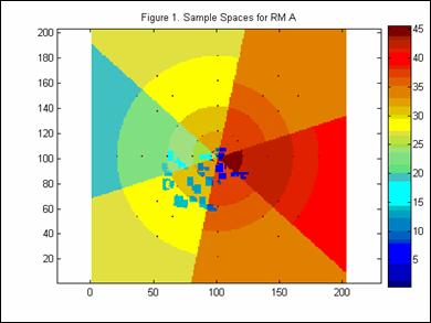
Each color in the figure denotes a particular sample space of RM A. Note that they very both with azimuth and distance (the transmitter resides at the center). 4 azimuth configurations and 6 distance ranges were sampled. A pseudo relation of the kth sample space SSk is defined as
SSk: {Indoors? AND φ < φok AND dlk < d < duk} (3)
where Indoors? is the implied binary relation, φ is the azimuth, φok is the azimuth threshold, d is the distance, and dlk and duk are the limits of the distance range.
Each sample space has a one to one correspondence with a prediction region. The predicted power Prk of the kth prediction region PRk relates to the distance through
![]() (4)
(4)
Here, Ck is a constant that is based on the average power Pavek accumulated from SSk and the distance do half-way between dlk and duk. Ck is defined as
![]() (5)
(5)
Equations (4) and (5) convey the relation between the analysis and prediction of the model.
Building Compensation:
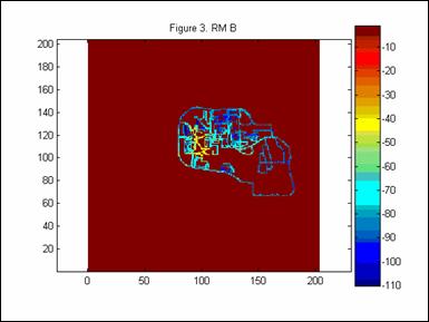
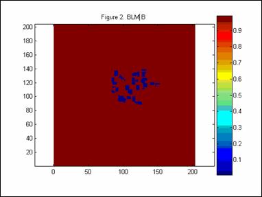
An integral part of the described model was defining the sample spaces and prediction regions with respect to building locations. To determine this component, idealized building location maps (BLM) were created as MATLAB matrices for each corresponding RM. Each element of the BLM and RM matrix have the same longitude and latitude. From this, it can be easily determined whether an element in RM falls on a building. Figures 2 and 3 compare BLM B with RM B.
The BLM’s were created using the MATLAB function imread with the provided bitmap graphic of the Georgia Tech campus [2]. Algorithms were then implemented so that the BLM’s were scaled appropriately and given proper coordinates.
Results:
Below are images of the prediction for RM A, RM B, RM C, and RM D.
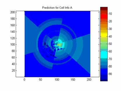
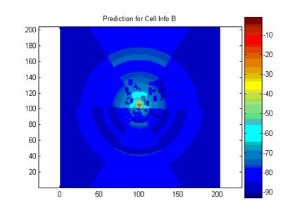
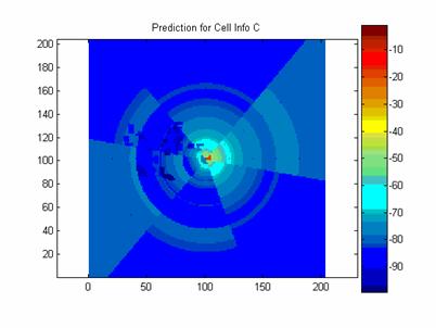
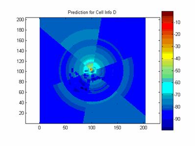
Executing the model with RM A, RM B, RM C, and RM D produce a mean of 0.9 dB and a standard deviation of 9.8 dB.
Conclusions:
Although the model proves to produce constructive results on the maps tested, its implementation onto a nationwide network might be hard to realize. The model relies on power readings that are taken from the Georgia Tech campus. If the terrain of interest was much different, the samples determining the model’s parameters would not be relevant. For a company to fully exploit the models utility, samples would have to be taken. This may be an expensive prospect, especially on a nationwide network.
Although the models direct implementation might be implausible, it provides useful information. In the process of designing the model, an average value of the loss of a signal in a building at a certain distance was found. This value also depended on antenna and signal parameters, but conclusions could be drawn to factor into other path loss models. The method for reproducing effective MATLAB data from satellite imagery might also serve as some purpose. Another product of the model’s design was insight into losses with respect to the azimuth. The gain pattern of any antenna can be theoretically produced, but the model outlines a means to test the antenna’s realization.
[1] Rappaport T. S. “Wireless Communications and Practice” 2nd ed. ISBN: 0-13-042232-0