Indoor/Outdoor Propagation Modeling on Georgia Tech Campus
Steven Lansel
Introduction
In today's society, cell's phones are everywhere and allow millions of people to communicate no matter where they are. However, cell phone users frequently complain of poor service and dropped calls. It is clear that this issues is very important to consumers since most of the marketing efforts for cell phone services focus primarily on the supposed strength of the company's cell phone coverage.
The main issue with cell phone use is how the strong the signal is at a given location. In order to better design a network for cell phone use, engineers must be able to predict the strength of a signal at multiple locations. Users often demand that their phones work in places that cause problems for electromagnetic propagation such as deep inside buildings or near large walls that may cause shadowing or reflections. Complex models are needed to predict the strength of a sent signal at all of these locations. Better propagation modeling will allow companies to increase the quality of their service at a lower cost, which could win over thousands of consumers and millions of dollars. The problem is nearly equivalent to the increasingly important issue of electromagnetic propagation of signals for wireless data networks.
Combining Received Power Map and Satellite/Building Mask Images
First, I attempted to combine all of the received power maps and the building mask image. The idea was that this would allow me to get a better picture of how buildings and other obstacles were affecting the signal strength and also to determine which readings were made indoors.
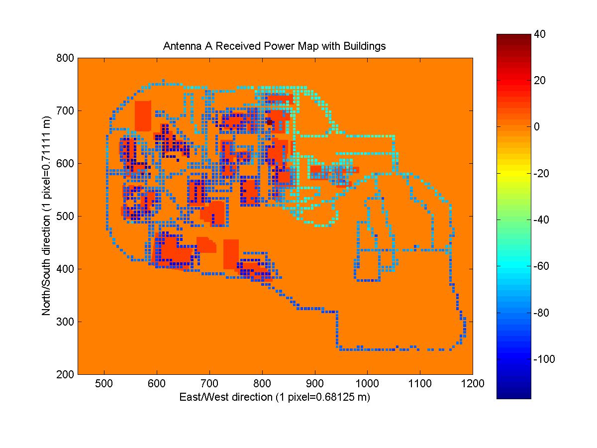
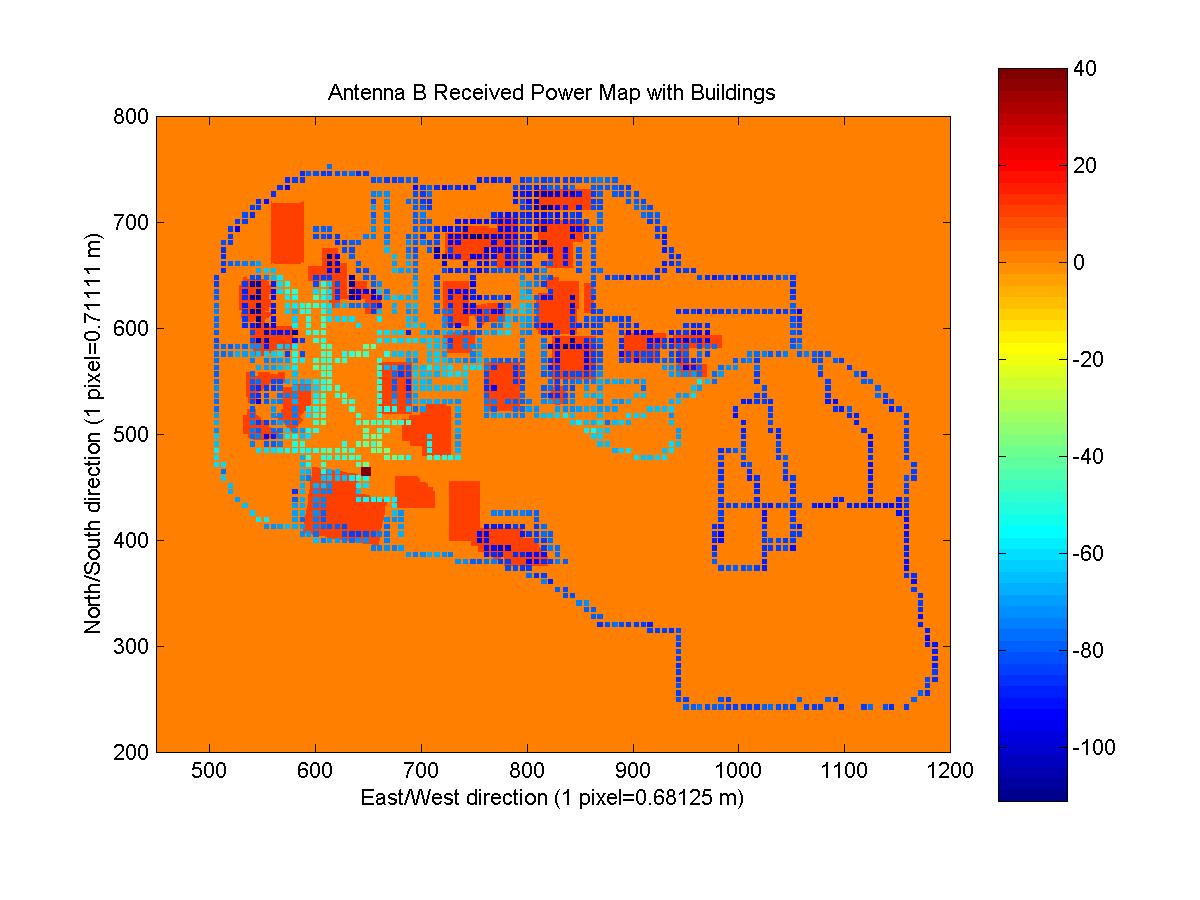
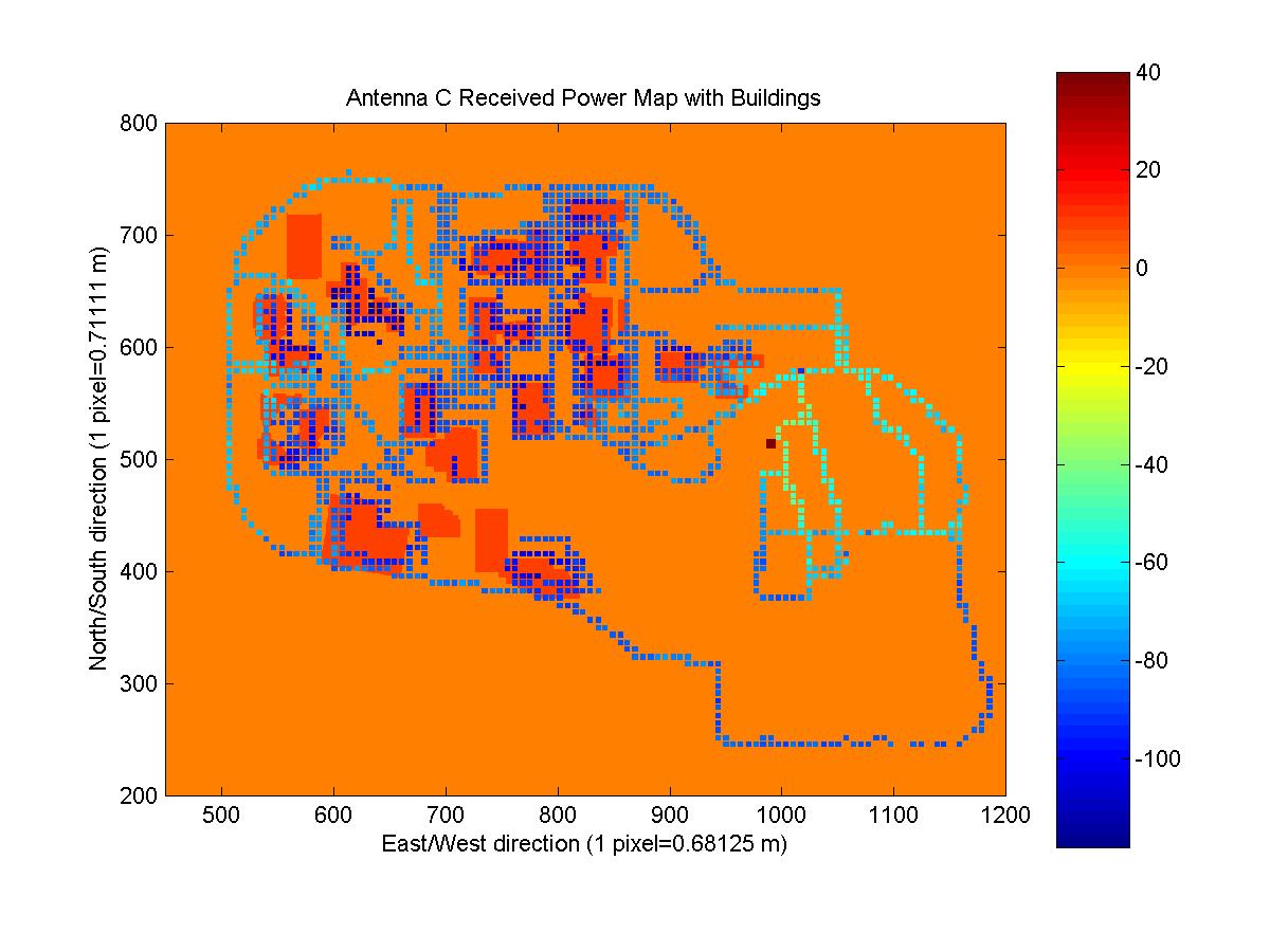
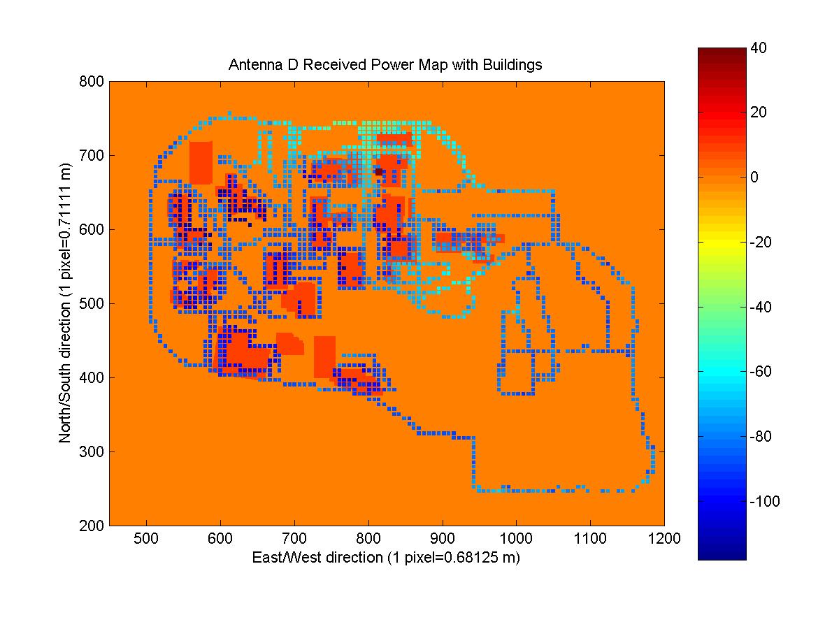
Instead of taking each received power map and resizing and positioning it until it appeared to match up with the satellite image, I tried a more scientific approach. With my own GPS receiver, I obtained two coordinates at locations that I could easily pick out on the satellite image. I chose the Van Leer parking lot and the corner of Peter's Parking lot (NW corner of the tennis courts). Knowing the location of two points on both images was necessary so that the location and scale for both the horizontal and vertical components could be matched properly. From the satellite image, I picked the pixels that correlated with the location of my measured coordinates. Using the longitude and latitude coordinates of the upper left and lower right pixels of each received power map, I was able to scale and position each received power map over the satellite/building mask images. The four images below are the resultant images (they can be clicked on to go to the full image, as well as all of the images in the report). The antenna location is marked with a square of value 40 and buildings are outlined with a value of 20. The code that generated the maps is CombineMaps.m. I created matrices that mapped the coordinates of each ReceivedPowerMap to the coordinates of the satellite and building mask images.
Dependence on Azimuth
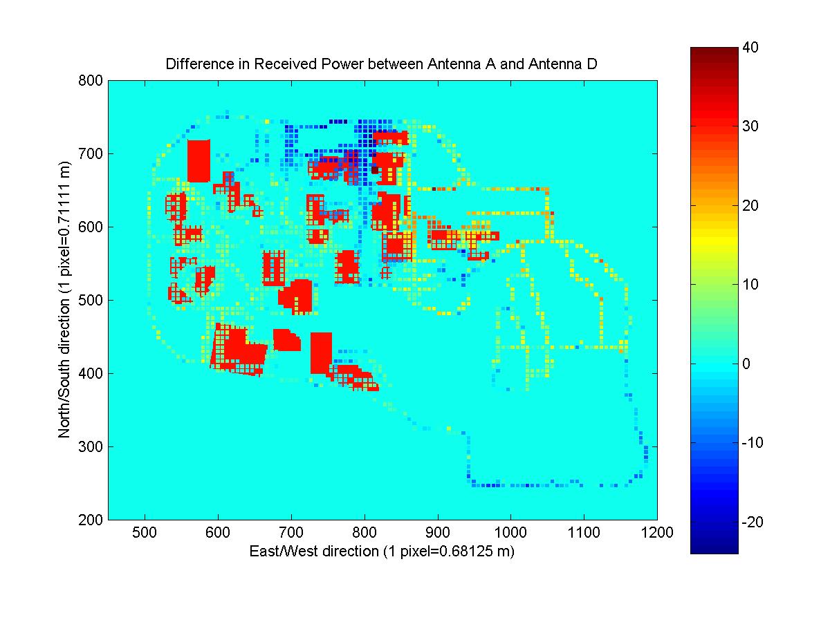
Since maps antennas A, D, and E; antennas B, F, and G; and antennas C and H, only differed by the azimuth, understanding how the gain of the antenna is affected by its orientation is critical. I noticed that the difference in the azimuth angles was always approximately 120 degrees (measuring the acute angle). Knowledge of how the gain of the antenna varies with azimuth wasn't given, so it was difficult to take this difference into account. But I realized that antennas A and D are identical except for the change in azimuth of 120 degrees. Therefore, any change in the received power maps should be a result of the change in azimuth. The following image shows the difference in the received power for antennas A and D, which is due to the azimuth.
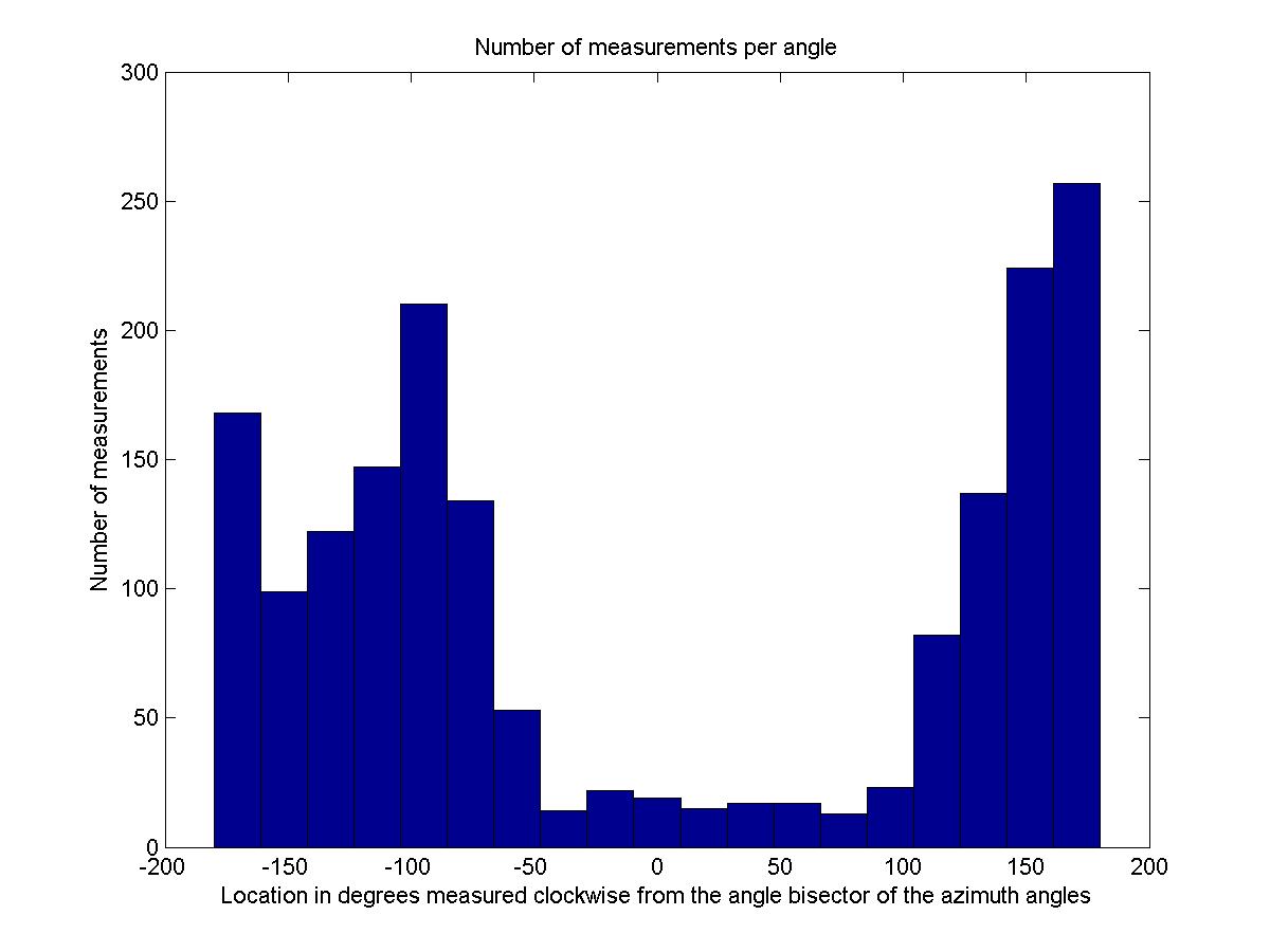
I calculated the difference in the received power due to the change in azimuth. For every point that had a measured value, I calculated the angle to the antenna relative to the angle bisector of the two azimuth angles. This way I could determine the variation in received signal strength as a function of angle since the effect of the change in azimuth has different effects depending on the location. The data is presented below on the left. The data was divided into 20 equal intervals and then averaged to generate the function shown in the image that approximates the change in gain due to angle. The image on the right shows the number of observations that were averaged for each point, which gives some indication of how reliable the resultant function should be.
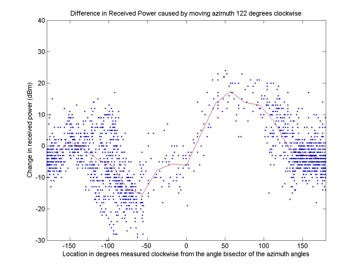
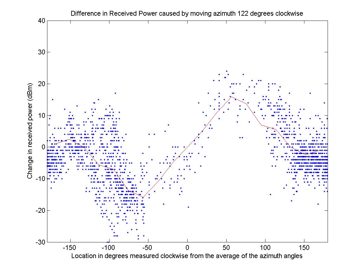
Looking at the function we have an approximation of the change in gain due to the angle. The function approximately passes through 0 at an angle of 0 and at angles of +/- 180 degrees (when the observed data is measured along the angle bisector of the azimuth angles), which is expected. Also the function has maximum and minimum at +/-60 degrees, which corresponds to where the azimuth of one of the antennas lies. However, using symmetry we can improve on the function by noting that due to symmetry the function should be odd (which is why I measured the angle from the bisector of the azimuth angles). I forced the function to be odd and increased its accuracy by averaging the absolute value of symmetric intervals. The following image shows the improved angle function. The function is indeed odd, periodic, and passes through 0 at 0 and +/-180 degrees. The code that generated the three plots is Angle.m. I wrote angleFactor.m, which is a function that gives the value shown below for any input angle (interpolated with straight lines between the known data points given by the averages).
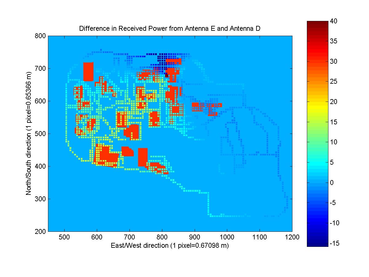
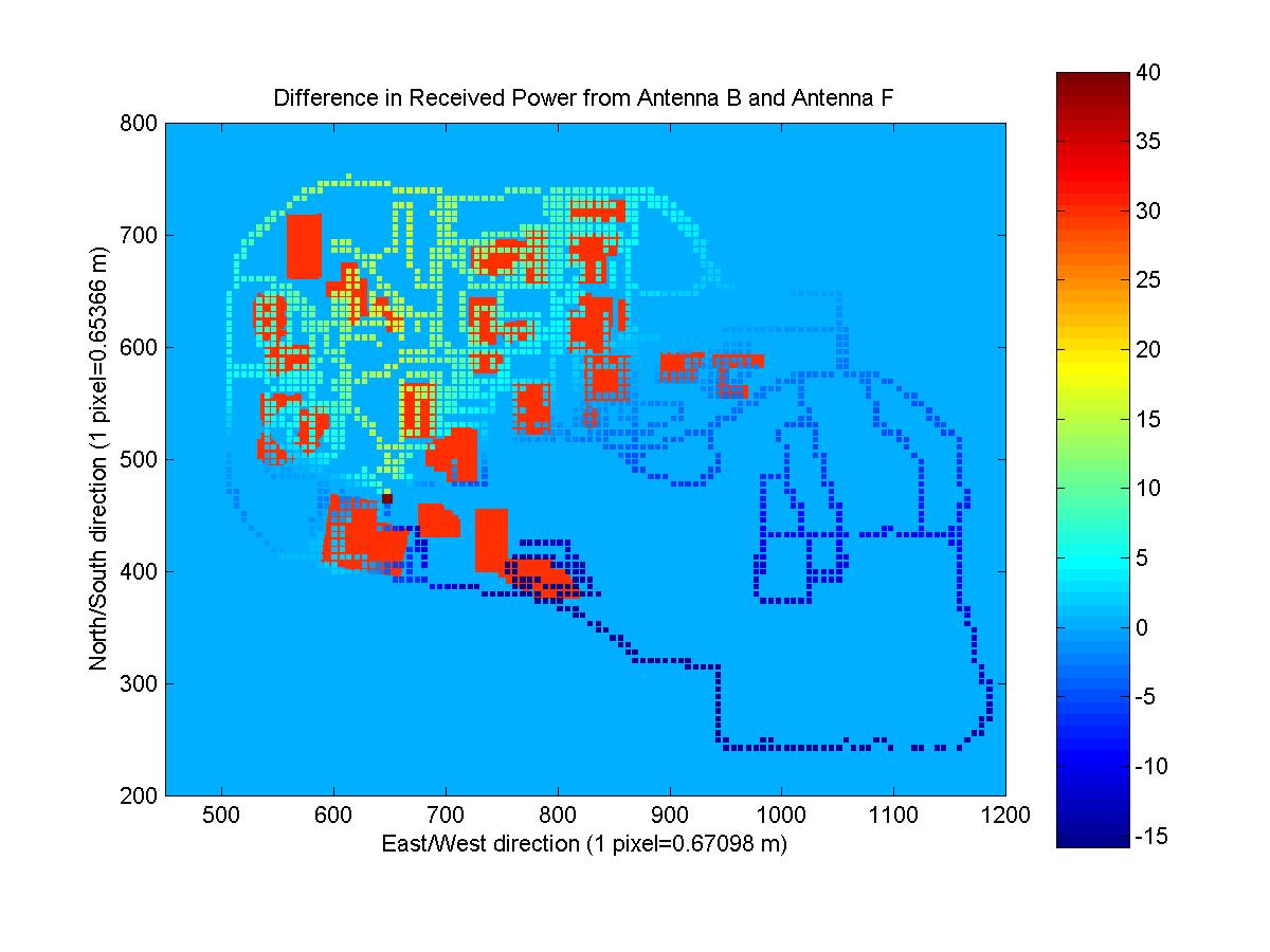
I used this angleFactor (difference in gain due to a change in azimuth angle of 120 degrees) to change all of the given measured data into predicted data for the new antennas. The difference in the received power maps is shown below for three different pairs of antennas. You can note that there is loss along the direction of the azimuth of the given antenna and gain along the direction of the azimuth of the unknown antenna.

Path Loss Calculation
Thus far, I have used the given data to predict the value of the received power for the unknown antennas but only at locations where previous measurements were given. Since it was specified that we would need to predict the received power at all locations on the map, a different method was needed to predict the rest of the points on the maps.
I decided to use path loss exponents (or something similar) to predict the remainder of the points. First, I divided the points into two sets dependent upon whether they were inside or outside. I used the look-up tables that I created outlined in the first section to check if a given pixel on the received power map was inside a building or not. After separating the two sets of data, I was able to calculate the distance from each point on the map to the antenna location. A plot of both sets of data vs the logarithm of the distance between the transmitter and receiver is shown below. I performed a linear regression on both sets of data (after taking the logarithm of the distance so in actuality it is an exponential regression), which is also shown in the figure below. Since the input power into antenna B was different from the other antennas, I adjusted the received power from antenna B so that it could compare directly to the other data. The code to generate the data and the regression is pathLoss.m.
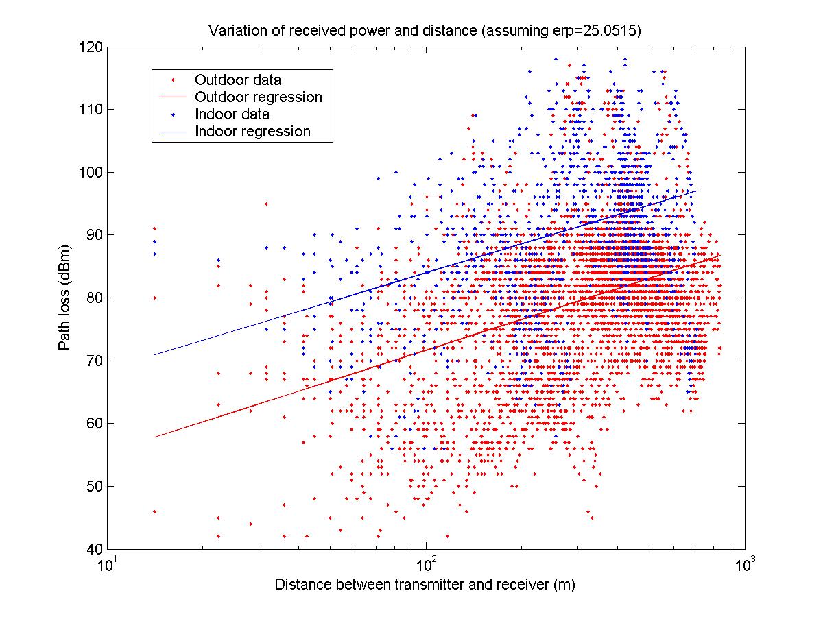
Although performing a linear regression and how I used it is slightly different than just finding the path loss coefficient, it will generate improved predictions. The difference is that the linear regression may not predict a reasonable path loss for small distances (the regression may not actually go through the origin), but since most of the data is at a large distance from the antenna the increased accuracy of the regression at large distances is more important.
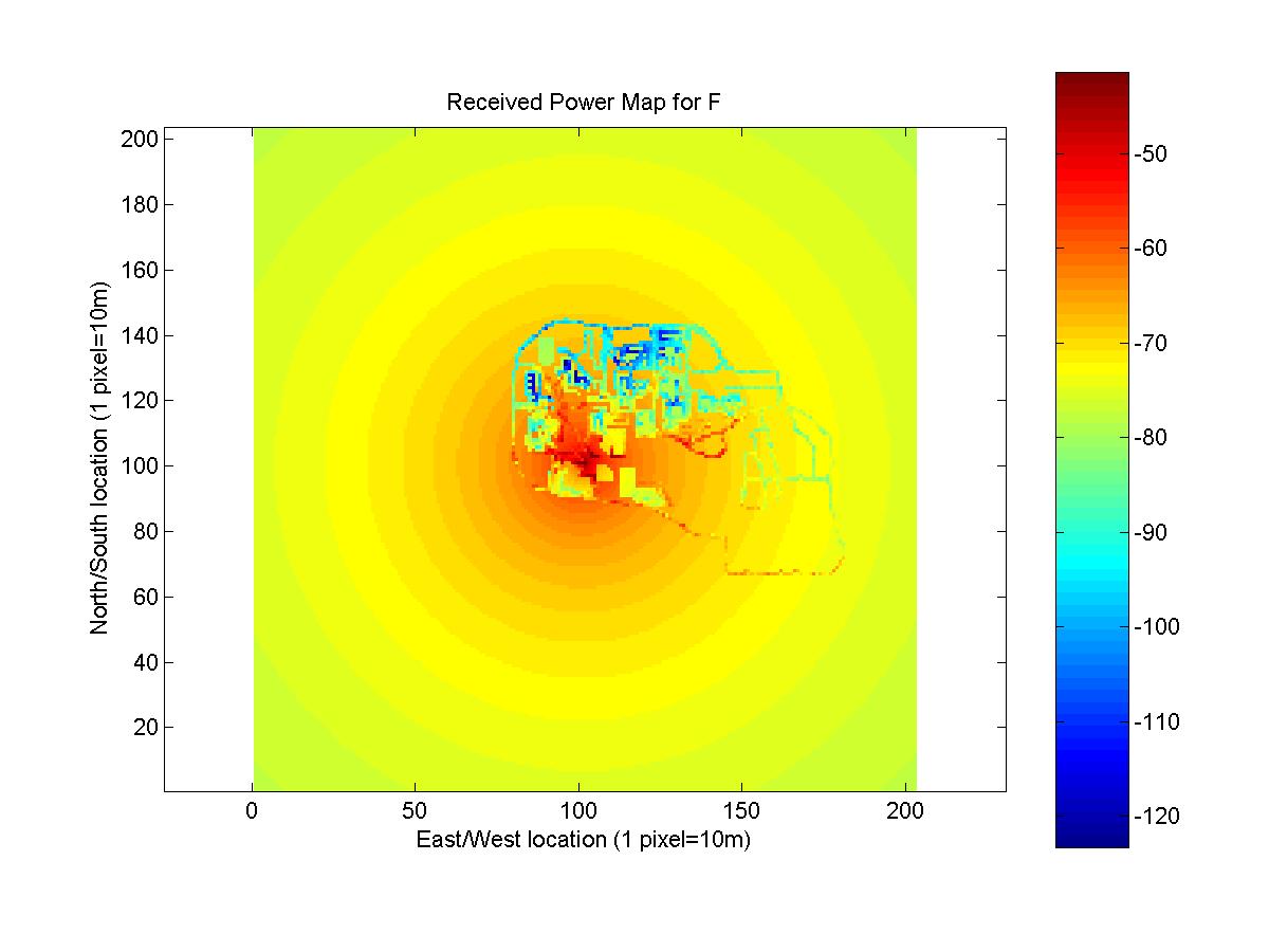
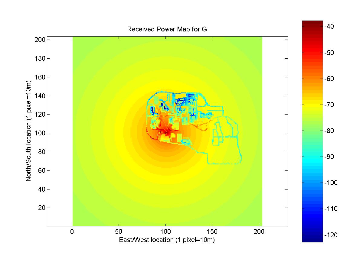
With the path loss regression, I predicted the received power at all of the unknown points for each of the maps (points where a measurement was not taken for the corresponding known antenna). For each point, I calculated the distance and found the corresponding path loss from the regression depending on if the location was inside or outside. I added approximately 12.94 dBm to each measurement for antennas F and G since the input power is higher for these antennas as opposed to the other antennas, which were used as a basis for the regression. The code that generates the maps using the azimuth and path loss calculations is final.m.
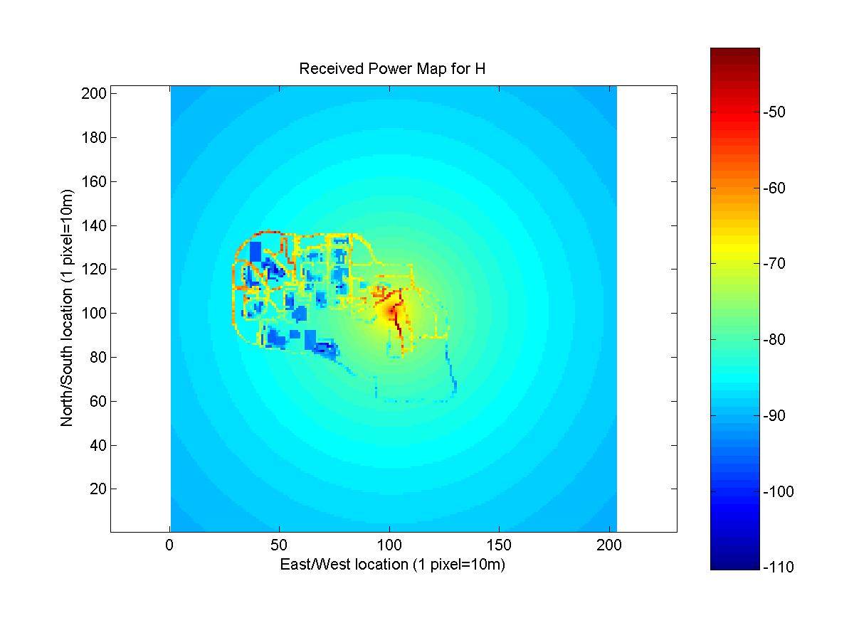
Conclusion
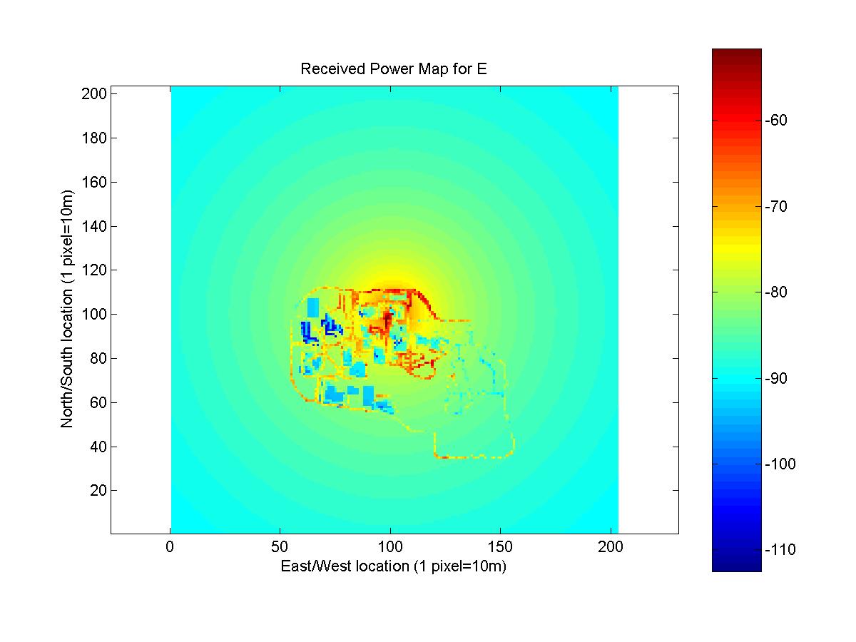
The predicted received power maps for antennas E, F, G, and H are shown below. The data for the maps is Lansel_Steven.mat.
Two different methods were combined to generate the maps. Knowledge of the change in gain as a function of angle, was used to predict received power for points that had measurements for antennas with the same location but different azimuth angle. This method has limited use in practice. If data exists for an antenna at a current location, a company could use this method to predict effects of changing the azimuth of antenna. The method gives no method to predict received signal strength if no existing data is used and cannot be used to determine the impact of changing the location of an antenna or adding a new antenna.
A linear regression similar to a path loss exponent was used to predict the received power at locations where no prior measurements exist. This general method can be used in practice where the particular regression constants (path loss exponents) are changed due to the particular environment of the antenna. A disadvantage of the method is that the only information included in the calculation is the distance to the transmitter and whether it is inside or outside. There is no difference between two locations that are equidistant from the transmitter where one lies directly behind a building and a location with a line-of-sight to the transmitter. Further factors could be included in the calculation by calculating multiple path loss exponents depending on additional factors other than simply whether the location is inside or outside.
My composite method of prediction cannot be compared with the known received power maps for Antennas A, B, C, and D since all of the measured points match-up exactly. Therefore, the method inherently has a mean and standard deviation of 0 when compared to these maps since their data was directly used in the process of predicting the other maps.