

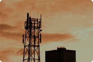
Cell phone masts cost upwards to a million dollars.
Image provided courtesy of FreeFoto.com
Within the last two decades, the cell phone industry has boomed. Networks have spread from flat, densly-populated cities to remote landscapes, deserts and villages in Africa, Asia, and South America. In some areas, cell phone development is the driving force of the local economy.
Cell phone transmitters, however are quite expensive, costing profit-minded companies millions of dollars to construct. In remote areas, where there are few people, it is necessary to deliver as much service from as few towers as possible, in order to maximize this profit. Therefore, precisely modeling for complex, large-scale landscapes is necessary, when dropped deciBels translate directly into lost revenue.
Due to the complexity of undeveloped terrain, the standard models of free space path loss are less accurate in places. full of rocky canyons and forested wilderness. So to accurately model these areas, more complicated properties of radio waves such as diffraction needs to be accounted for as well

Figure 1 - A visual description of the variables used to model the given terrains.
For this assignment, an empirical model for four outdoor terrains was developed using reception samples from four other terrains. To utilize the data, a partition scheme was generated to relate sizdifferent variables to the received power at a given point:
- D - Distance
- θ - Elevation Angle
- α - Proximity to azimuth angle
- δ - Line of sight
- V - Diffraction level
- C - A path loss constant
A linear partition model was chosen to simplify calculations in application, while the variables were chosen to best accomidate free space attenuation and geometrical effects.
Free Space Attenuation
The degradation of a propagating signal through space is most popularly modeled through the Friis Equation(1) for link budgets,
in which a given signal degrades exponentially, fit by a path loss exponent. However, when modelling in decibels, this
parameter is simply multiplied against the distance in log space. So while Friis equations can better account for path loss
over space, using distance as a parameter can adequately measure free space attenuation, while the portions of
the link budget equations dependent on unchanging parameters such as antenna gain can be accounted for with a constant
parameter. Also, the Azimuth angle of the transmitting antenna was considered because the orientation of an antenna affects
reception. If the angle between the transmitter and receiver is near the azimuth angle, this value is set to "one", and
"zero" otherwise. Finally, eirp, or isometrically modeled transmitted power was subtracted from the equation constant to
allow for different transmission strengths.
Geometrical Effects
Uneven terrains complicate microwave modeling, but they can be approximated in several ways. A boolean (1 or 0) value was
assigned for line of sight, one if blocked, zero if within the line of site, because reception is weaker in the shadow of an
obstructing object. The elevation angle between the transmitter and receiver was also used as a parameter, because at higher altitudes
over open terrain, signals are often better spread and are more likely to have line-of-sight. Finally, diffraction was
accomodated for, and is discussed in greater detail later.
Over 100,000 samples were used to fit the variables by plugging them into the standard "Normal Equations", a set of equations for fitting data into correlations(2). By averaging the results obtained from each terrain analysis, the following formula was determined:


Several models exist for diffraction. However, the model must be simple, because to apply this model in real-world situations, it must be feasable to calculate this diffraction in a timely manner, so that larger areas can be surveyed more quickly. Also, it must be represented as a scalar value that it can be fitted into a linear partition model.
 (Eq 1)
- v=0 if there is line of sight, or if the antenna separation distance is close relative to the height of any obstruction
- The "obstructing object" is modeled by the largest blocking object between the transmitter and receiver.
Figure 2 - The simplified diffraction model used to calculate v.
A fortunate aspect of Fresnel Parameters is that for values above 1, the relationship in log space (dB) between v and extra path loss is linear(3), allowing it to be successfully adopted into the partition model.
Using a Fresnel Parameter for a single object to replace diffraction over a large range of terrain is not nearly as accurate as implementing mathematical signal propagation models such as the Somersfield or GTD equations, but the capabilities of the computers must be considered. Calculating "v" alone accounts for over 90% of the simulation time for the program used to simulate this model. Using a more accurate model would make calculations inconveniently long.

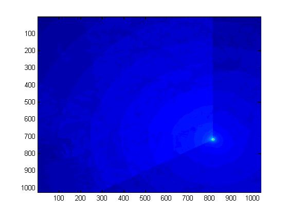
Four cell sites (A, B, C, D) were provided with measurements, along with four other sites without measurement. The model for propagation was generated using a C program, main.c. The model was simulated for all eight cells
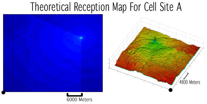
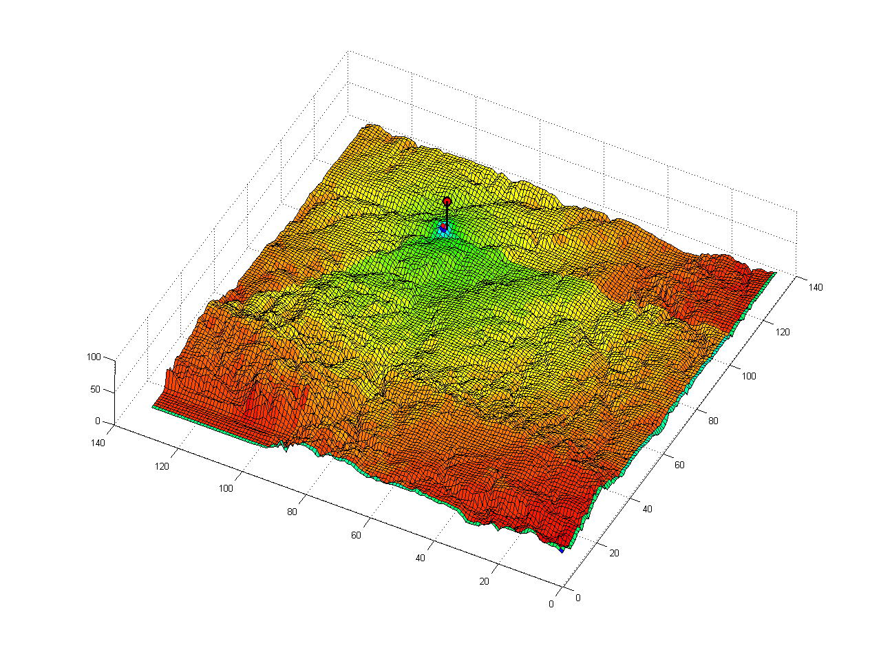
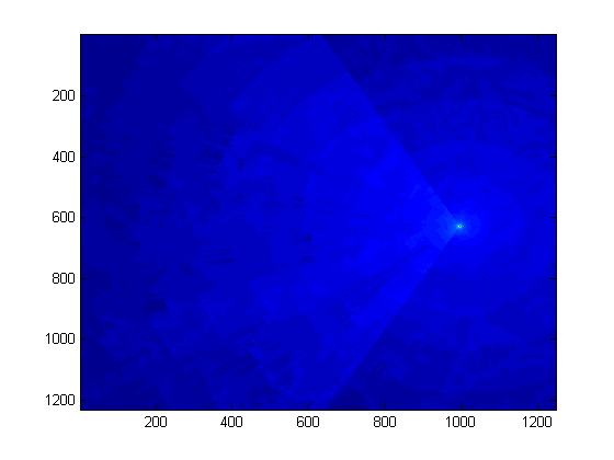
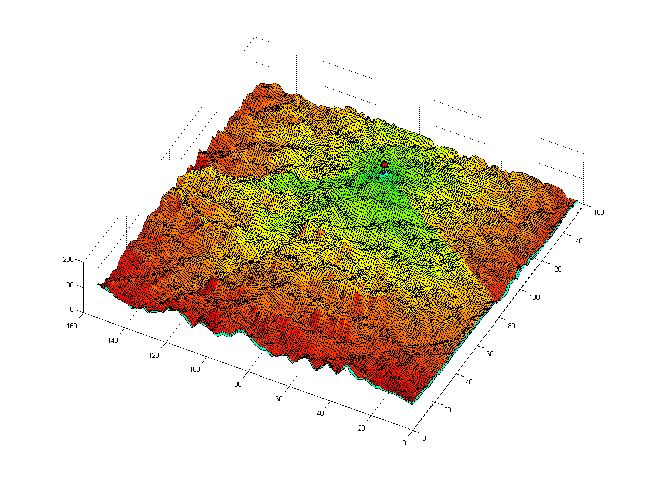
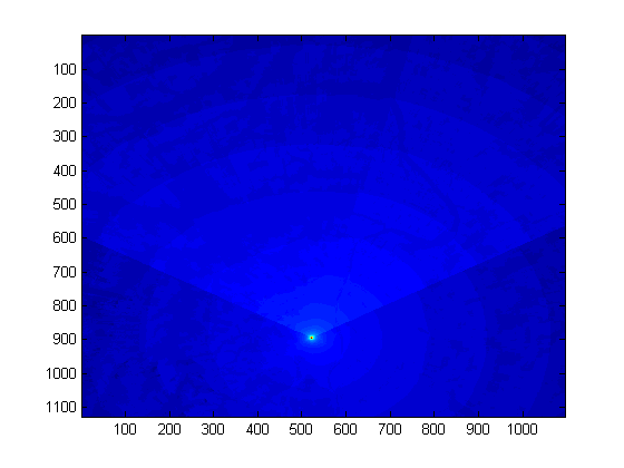
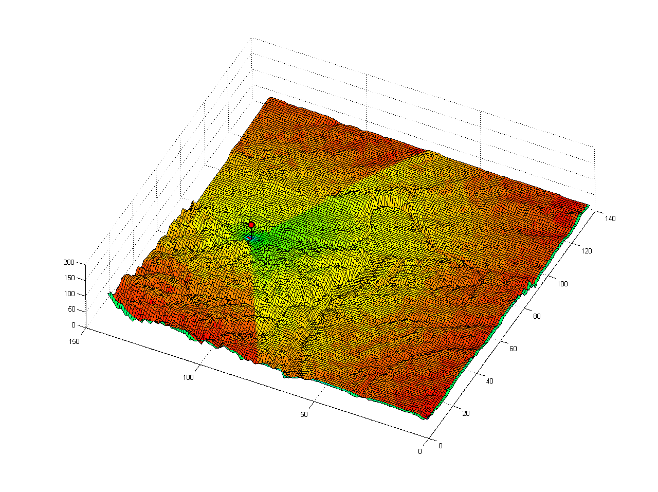
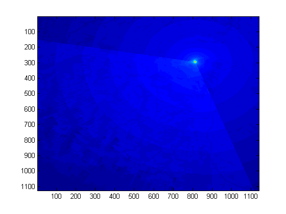
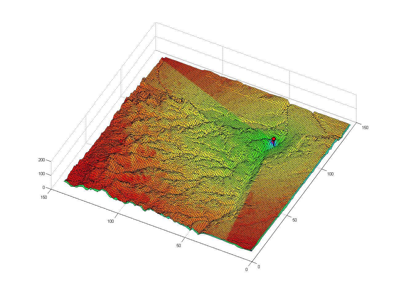
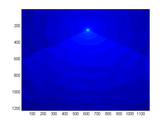
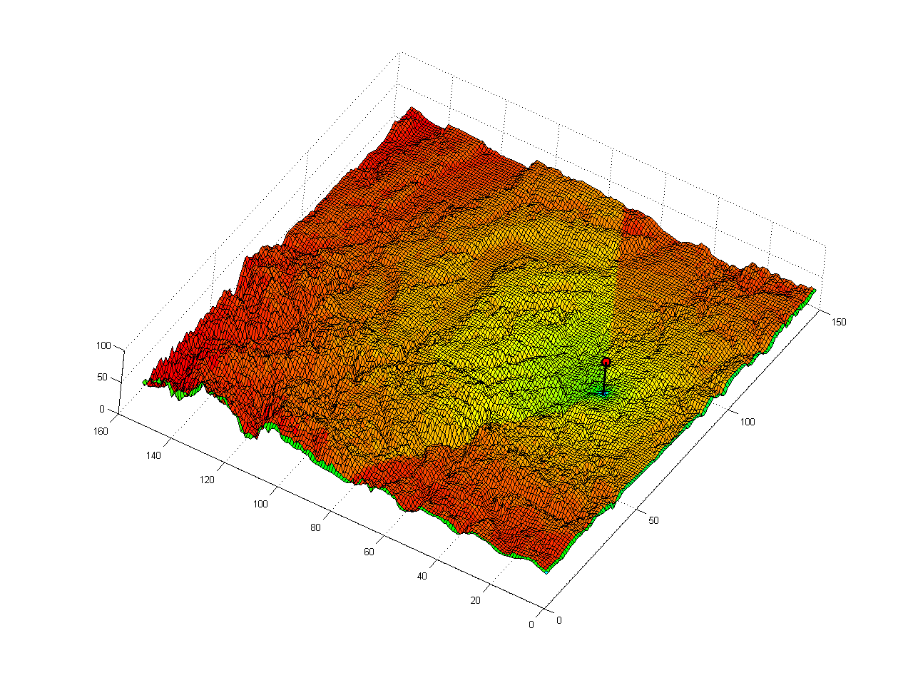
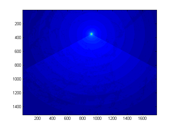
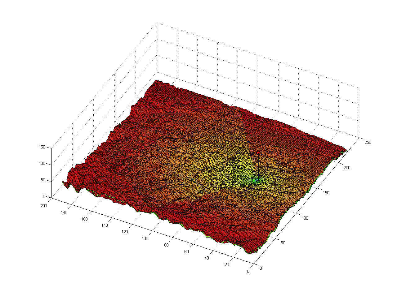
Figure 3 - Calculated reception map for cell site A, projected onto a 3d rendering of its terrain.
With theoretical values for the four maps, the results were checked against the actual, measured values, to generate mean and standard deviations for the model. The results of this comparison are shown below.
Model Accuracy Analysis| Cell Site | Mean Error | Std Dev |
| A | -2.40dB | 7.54dB |
| B | 2.49dB | 8.60dB |
| C | 2.64dB | 7.48dB |
| D | -1.65dB | 8.77dB |
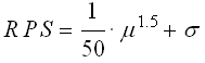
This resulted in a total RPS (Raw Performance Score) of 8.2 using the following formula:
The model presented is not a general solution for diffraction or microwave propagation. It is an empirical correlation that is meant only for the area being measured, so applying the formula used elsewhere would be fruitless. However, the process used, generating partition models based on existing sampled data, can be applied to not only diffraction modeling but any observasional research, and the techniques used to develop the partitions can be applied at other sites for similar results.

Source Code
- main.c - Program used to calculate partition statistics
- simulate.c - Program used to apply model to cell sites
References
- Cheng, David K. Field and Wave Electromagnetics. 2nd ed. Reading, Massachusetts: Addison-Wesley Company, 1992. 639-643.
- Durgin, Greg. "Measurements and Models for Radio Path Loss and Penetration Loss in and Around Homes and Trees At 5.85GHz." IEEE Transactions on Communications 46 (1998): 1484-1496.
- Willis, Mike. "Diffraction Over Terrain." Propagation Tutorial. 24 Apr. 2006 <http://www.mike-willis.com/Tutorial/diffraction.htm>.
Extra Images
- Site A - Measurement Image, 3d Rendering
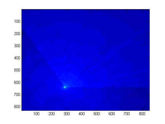
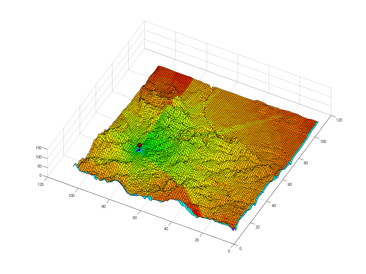
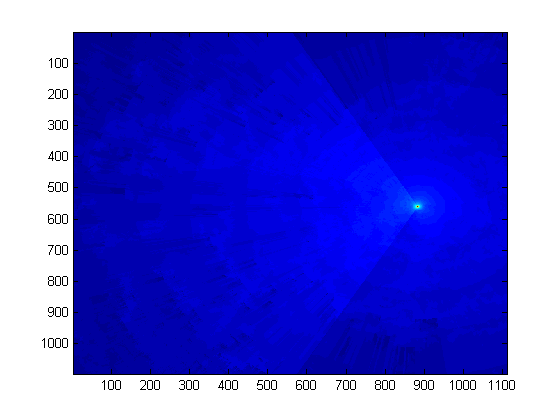
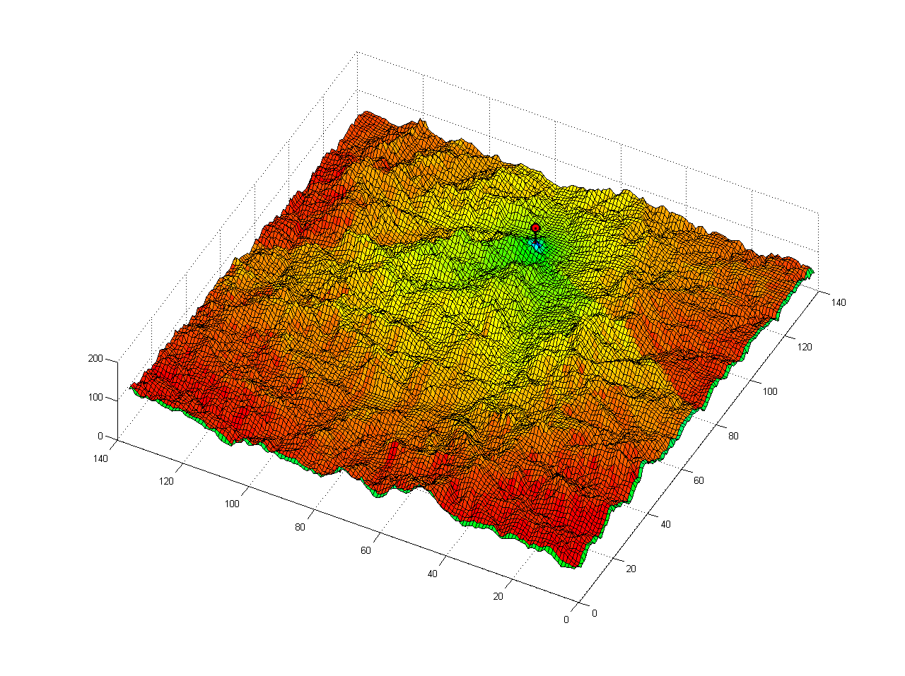
- Site B - Measurement Image, 3d Rendering
- Site C - Measurement Image, 3d Rendering
- Site D - Measurement Image, 3d Rendering
- Site E - Measurement Image, 3d Rendering
- Site F - Measurement Image, 3d Rendering
- Site G - Measurement Image, 3d Rendering
- Site H - Measurement Image, 3d Rendering