Signal Propagation Modeling Using
Fourier Synthesis to Optimize the Friss Free Space Equation Through Iterated
Variation of Parameters.
Andrew Seltzman
Georgia Institute of Technology
gtg135q@mail.gatech.edu
(Dated:
I. Introduction
Signal propagation modeling plays a vital role in modern microwave communications as variations in signal strength due to antenna pattern and terrain effects can influence the reliability and fading of a given radio link. With the advent of modern satellite generated terrain maps, it is possible to accurately derive a model for terrain diffraction effects based on surface slope and receiver location. The use of a simulated received signal strength model will allow selection of a transmission system’s characteristics and location to optimize coverage thereby minimizing signal dropout potentially saving millions of dollars over the design lifetime of the system.
II. Propagation Model
The basic model (1) of RF propagation relies on the Friss free space equation, as a function of distance, gain, wavelength, and effective radiated power, assuming even terrain effect represented in the path loss exponent n, and isotropic power radiation by the transmission antenna.
![]()
This model can be further improved by analyzing the azimuthal and elevation power distributions of the transmission antenna as well as terrain diffraction effects allowing a higher accuracy in signal strength estimation. The improved model (2) includes a terrain diffraction term calculated from the angle of incidence between an incoming plain wave and the slope on the surface of the terrain.
![]()
It is now possible to optimize the
model by solving for the azimuthal and elevation power spectrum with a correct
distribution function generated by a Fourier synthesis. Since any arbitrary
function can be synthesized with a Fourier series it is no longer necessary to
know the form of the function to be generated. The directional gain of an
arbitrary antenna radiation pattern can be represented by a suitable Fourier
synthesis involving a series of superimposed cosine functions (3) with
optimized gain coefficients ![]() .
.
![]()
The standard deviation (4) used to
check the accuracy of the propagation model is a function of ![]() for each measured
point on the map, allowing a global minimum in
for each measured
point on the map, allowing a global minimum in ![]() to exist for each
point. Since a global minimum exists for each individual point, a global minimum
exists for the function.
to exist for each
point. Since a global minimum exists for each individual point, a global minimum
exists for the function.
![]()
The presence of a function with a
global minimum allows optimization of the model by using variation of
parameters to minimize the standard deviation function. Variation of parameters
utilizes the zero crossing of the first derivatives of a multivariable function
to determine the global minimum and is routinely utilized in optimization
problems. The standard deviation with respect to a given variable ![]() is determined
numerically and subsequently minimized. By the definition of multivariable
derivatives (5), the exact derivative of the standard deviation occurs when the
partial derivatives of a function equal 0 simultaneously.
is determined
numerically and subsequently minimized. By the definition of multivariable
derivatives (5), the exact derivative of the standard deviation occurs when the
partial derivatives of a function equal 0 simultaneously.
![]()
Therefore the global minimum of a multivariable function occurs when the function is simultaneously minimized with respect to each of its variables.
Normally,
the global minimum of the function would have to be computed by simultaneously
adjusting the individual variables to the minimizing valve, however if the
derivatives ![]() are linearly independent, the minima of the function can be
found by iterating variation of parameters on each variable in succession
without invalidating the determined minimizing value of previously determined
variables.
are linearly independent, the minima of the function can be
found by iterating variation of parameters on each variable in succession
without invalidating the determined minimizing value of previously determined
variables.
Exploiting the linear independence between cosine terms (6) in the Fourier series, variation of parameters can be applied to minimize the standard deviation of the propagation model with respect to a given Fourier coefficient without requiring successive corrections to previously determined coefficients of a lower order.
![]()
An optimum model for relieved signal strength can therefore be computed by using variation of parameters to minimize a models standard deviation during successive addition of Fourier coefficients. The resulting series can be used to precisely model the antennas radiation pattern as derived from the measurement data provided on the map.
Further optimization of the propagation model can be accomplished by modeling terrain reflection and shadowing. The X and Y slopes of the terrain can be calculated from the gradient (7), allowing the angle of incidence on the surface to be computed by subtracting the incidence angle from the angle of the slope.
![]()
Assuming vertical polarization, the component of the plane
wave in a given direction is multiplied by the cosine of the angle between its
incidence and the slope of the surface. The resulting function simulates the
doubling of a vertical polarized wave with a near tangential incidence at far
distances. The previous equation is added to the Y axis component and the sum
is added to the received signal strength, providing an approximate model of
terrain reflection and shadowing.
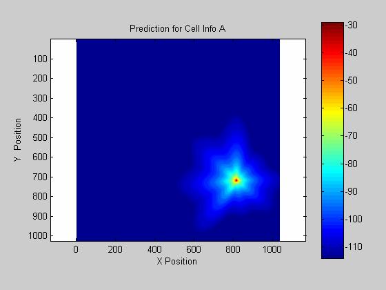
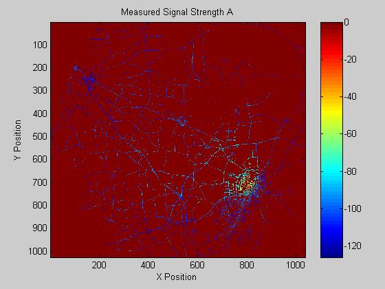
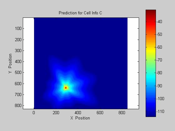
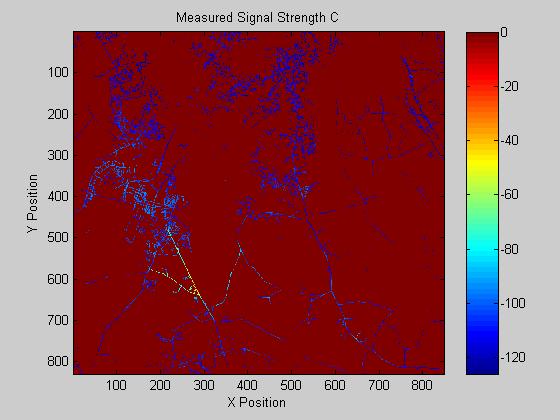
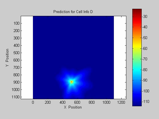
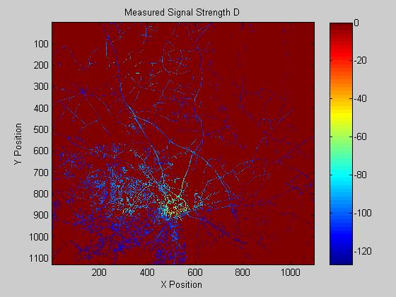
I. Predicted Signal Coverage
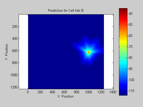
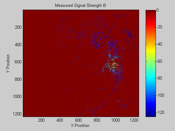
The provided 4 measurement and terrain maps were utilized to model the propagation of a plane wave across an uneven terrain. The resulting model provided both low standard deviation and mean error as given in figure 1. The four known coverage maps and their respective predictions are given below.
Site Cell_Info_A, mean of -6.76 dB, std dev of 9.45 dB
Site Cell_Info_B, mean of -0.06 dB, std dev of 7.62 dB
Site Cell_Info_C, mean of -0.55 dB, std dev of 7.44 dB
Site Cell_Info_D, mean of -5.89 dB, std dev of 10.58 dB
Average Error of (mean = 3.3 dB, sigma = 8.8 dB) for 4 site(s)
Raw Performance Score (RPS): 8.9
Figure 1. Propagation model accuracy.
II. Conclusions
The determined model accurately predicts signal coverage over uneven terrain, however it should be noted that due to the relative flatness of the maps in use and the optimization of the model, the terrain correction is negligible when compared to that of the antenna pattern and Friss free space equation. In these cased of open landscape and direct propagation over relatively smooth ground, more consideration should be given to the design of the antenna in order to insure proper signal coverage, however when used in a cluttered area such as a city or mountainous terrain a different model should be developed in order to provide accurate results.
This model can be used by cellular designers to provide insight into how signals from a given system will propagate allowing optimization of antenna pattern and election in order to provide best coverage and minimal signal dropout.
III. References
[1] G. Durgin “Overview of the Geometrical Theory of
Diffraction”
[2] G. Durgin “Large scale path loss” Class Notes, Spring 2006
IV.
Appendix A: Propagation Model Code
function [ret,model] = sprop(Cell_Info_X)
%propegation model
% usage:
% [ret] =
% Cell_Info_X = input struct
%
%
%warning off MATLAB:divideByZero
[M,N] = size(Cell_Info_X.terrain); %dimentions M rows(hight) by N columns(width)
azimuth = Cell_Info_X.cellSite.azimuth; %transmitter azimuth angle azimuth=0 on y+ axis
eirp = Cell_Info_X.cellSite.eirp; %transmitter EIRP
BSx = Cell_Info_X.cellSite.BSx; %transmitter x position
BSy = Cell_Info_X.cellSite.BSy; %transmitter y position
freq = 1e6*Cell_Info_X.cellSite.freq; %transmitter frequency in mhz * 1e6 Hz/MHz
cellSize = Cell_Info_X.cellSite.cellSize; %size of each pixel in meters
AGL = Cell_Info_X.cellSite.height; %antenna height AGL
terrain = double(Cell_Info_X.terrain); %terrain in meters ASL double format
ASL = AGL + terrain(BSy,BSx); %antenna height ASL
[FX,FY] = gradient(terrain); %X (L to R) and Y (T to B) gradients of terrain (slope in meters of elevation per pixel)
%Contants
c = 3e8; %speed of light
lambda = c/freq;
%variation of parameters data
%-----------------------------
Gr = 78; %Receiver gain
n = 1.86; %path loss exponent
gamma0 = 1; %azmuthial radiation pattern fourier coefficient F0
gamma1 = 0.022; %F1
gamma2 = 0.005; %F2
gamma3 = -0.017; %F3
gamma4 = 0.002; %F4
gamma5 = 0.0075; %F5
gamma6 = -0.002; %F6
gamma7 = -0.007; %F7
gamma8 = -0.009; %F8
gamma9 = 0.003; %F9
delta0 = 1; %elevation radietion pattern fourier coefficient F0
delta1 = 0.075; %F1
delta2 = 0.007; %F2
delta3 = 0.000; %F3
delta4 = 0.000; %F4
%terrain coefficients
terrv0 = -0.17;
%initilize prediction matrix
pred=zeros([M,N]);
for I = 1:N, %(width X(to right))
for J = 1:M, %(hight Y(top down))
r=sqrt((cellSize^2)*((I-BSx)^2+(J-BSy)^2)+(ASL-terrain(M,N))^2); %distance in meters to observer
phi=atan2(-(J-BSy),I-BSx)-pi/2; %angle with respect to phi=0 on y-axis -phi = cw, phi=-pi/2 for x, phi=pi/2 for -x
theta=atan2(terrain(J,I)-ASL,cellSize*sqrt((I-BSx)^2+(J-BSy)^2)); %elevation angle of incident wave
%azimuth patern factor
az=(gamma0-gamma1*cos(azimuth-phi)-gamma2*cos(2*(azimuth-phi))-gamma3*cos(3*(azimuth-phi))-gamma4*cos(4*(azimuth-phi))-gamma5*cos(5*(azimuth-phi))-gamma6*cos(6*(azimuth-phi))-gamma7*cos(7*(azimuth-phi))-gamma8*cos(8*(azimuth-phi))-gamma9*cos(9*(azimuth-phi)) );
el=(delta0-delta1*cos(theta)-delta2*cos(2*theta) ); %elevation pattern factor
Sy=abs(cos(phi)); %signal y component cos since phi=0 on y axis
Sx=abs(sin(phi)); %signal x component
% vert comp on x slope vert comp on y slope
terrv= ( Sx*cos(-sin(phi)*atan2(FX(J,I),30)-theta) + Sy*cos(-cos(phi)*atan2(FY(J,I),30)-theta)); %terrain diffraction factor
point = eirp + terrv0*terrv + Gr - 20*log(4*pi/lambda) - 10*n*log(r)*az*el; %calculate recieved signal strength
if point < -114, %limit value to above -114dB
pred(J,I)= -114;
else
pred(J,I)= point;
end
end
end
model=int8(pred);
ret=Cell_Info_X.cellSite; %return transmitter attributes