
ECE6390 Satellite Communications and
Navigation Systems
Radio Location Scavanger
Hunt 1
SARSAT Rescue
1. Project Statement
A large commercial jet has made a
crash-landing somewhere in the
2. Measurements
The following data is the measured carrier frequency as a function of time. The receiving satellite is making an upwards orbital swing (from south to north) and is riding the -76.000˚ longitude line.
Figure 2.1 Measured carrier frequency by
the satellite
3.
Code Description
The
code that was simulated for this problem was splitted
in two parts:
- The first part finds the latitude of the position based on the statistics collected at
the satellite. For that we computed the derivative of the Doppler shifted
data and tooked its maximum absolute value.
- The second part finds the longitude a recursive method that simulated the Doppler shift
by the satellite
4.
Calculations
The latitude
is found by taking the time derivative of the provided data set. However,
before the derivative could be found, the data had to be filtered. Different filters were tried, but the
averaging filter proved to be the best. The final step was to find the
time where the derivative was at a minimum (or max of the absolute value). Because
the data was still not smooth, all points with the minimum value were found and
the average time was used.
The
following is the filter implementation for smoothing the data:
SizeFreq = size(FreqData);
n = 10;
for a = (n+1):(SizeFreq(2)-(n+1))
SmoothFreq(a) = mean(FreqData(a-n:a+n));
End
SmoothFreq(1:n) = SmoothFreq(n+1);
SmoothFreq(SizeFreq(2) - (n+2) : SizeFreq(2)) = SmoothFreq(SizeFreq(2) - (n+1));
Figure 2.2 Derivative of the measured
data.
With
the data mostly smoothed out, the derivative was taken by calculating the
difference in the frequency vector divided by the time step. Then the derivative
data was plotted, it was noted that the curve was still not entirely smooth but
was good enough to get values from.
DF = diff(SmoothFreq)/dt;
DerValue = max(abs(DF));
Based
on the given satellite period and the time when the satellite sub point was
over the equator, the longitude of the transmitted signal was determined.
LatIndex = round(mean(AllElem));
LatTime = TimeData(LatIndex);
SatPeriod = 6119;
SatSecPerDegree = SatPeriod / 360;
Latitude = LatTime
/ SatSecPerDegree
The latitude found was: 25.7748˚
For the
longitude, an iterative method was used. The
latitude was then known from the previous part, so different longitudes were
guessed until the correct longitude was found.
This was accomplished by taking the latitude and trial
longitude and generating Doppler shift data based on the azimuth and elevation
look angles and the satellite’s velocity. The
data was then compared to the given data set by taking the derivative as was
done in the first part and comparing the minimum value to the value found from
the first part.
Starting at the longitude of the satellite (-76.00
degrees), different longitudes were tried
until a match was found.
The following is the section of the code that achieves this
calculation:
function [Longitude] = GenDop(TimeData, DerValue, Latitude,
Start, Step)
%satelite
speed
Vs = 7300; %km/s
Ts = 6119; %satellite period
SatDegPerSec = 360 / Ts;
%step through all longitudes
until the correct max derrivative is found
%if go directly from Start,
you get a divide by zero warning
for Longitude = Start-Step:-Step:-200
%Latitude
Le = Latitude * pi/180;
LsData = SatDegPerSec .* TimeData;
LsData = LsData *
pi/180;
%Longitude
le = Longitude * pi/180;
ls = -76 * pi/180;
%radius of the earth and satellite
re = 6370;
rs = re + 1000; %altitude
is either 1000km or 850km
%the perticular satelite we are using is 1000km
SizeLs = size(LsData);
%calculate the azimuth and elevation look angles
for n = 1:SizeLs(2)
Ls = LsData(n);
gamma = acos((sin(Ls)*sin(Le)) + (cos(Ls)*cos(Le)*cos(ls-le)));
El(n) = acos(sin(gamma)/sqrt(1+((re/rs)^2)-(2*(re/rs)*cos(gamma))));
Az(n) = asin(sin(abs(le-ls))*cos(Ls)/sin(gamma));
if Ls < Le
Az(n) = pi - Az(n);
end
end
%Change the Az
convention
Az = pi - Az;
%Calculate the preceived
satellite velocity
VsTime = Vs .* cos(El) .* cos(Az);
%Calculate the doppler shift
f0 = 406e6;
lam0 = (3e8)/f0;
Doppler = VsTime/lam0;
%Take the derrivative
of the doppler data
dt = TimeData(500) - TimeData(499);
DiffDopp = diff(Doppler)
/ dt;
%remove artifacts in the
derrivative (this may not be the best way to
%do this
SizeDiffDopp = size(DiffDopp);
for a = 2:SizeDiffDopp(2)
if abs(DiffDopp(a)-DiffDopp(a-1)) > 0.5
DiffDopp(a) = DiffDopp(a-1);
end
end
%Find the maximum of the calculated derrivative
DiffDopp = max(abs(DiffDopp));
%If the calculated value
is less than the real value, you stepped one
%too far in longitude. The signal is coming
from between that
%longitude and one step before that.
if abs(DiffDopp) < abs(DerValue)
break
end
end
The longitude determined by the
code was -78.8700˚
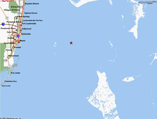
Figure 2.3
Approximate Location
The exact
location of commercial jet is found to be at the