By combining our dielectric material relationship, our definition of electric potential, and Maxwell's electrostatic equation, it is possible to derive a differential equation that relates space-varying voltage to the volume charge density of space:

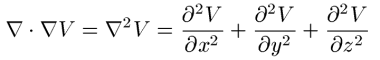
In words, this equation states the following:  the divergence of the gradient of voltage is proportional to the charge volume density at every point in space.  The operation involving the divergence of  the gradient of a scalar function has a special name in the physical sciences; it is called the Laplacian.  Thus, we could restate this equation in the following words:  the Laplacian of voltage is proportional to charge volume density.  The Laplacian operator occurs so frequently in electromagnetics and other fields that it has its own short-hand notation: .  The Laplacian operator for voltage is defined as follows:

Although the Laplacian has a compact, elegant form, it defines a multivariable partial-differential equation that can be quite difficult to solve.

The equation that relates the Laplacian of voltage to electrostatic charge has two names, depending on the presence of charges.  Poisson's equation is the name of this relationship when charges are present in the defined space.  To solve Poisson's equation, we require two pieces of information about the solution region of space: 1) voltage boundary conditions and 2) the charge distribution.  Laplace's equation is the name of this relationship  when there are no charges present and only requires information about voltage boundary conditions.  Thus, the two forms of this equation are

In this discussion, we will be focusing on the numerical solution of Laplace's equation, although it is very easy to extend the results to Poisson's equation.

Discrete Laplace's Equation

There are very few examples of electrostatic problems that can be solved using the analytic form of Laplace's equations.  Fortunately, we can recast Laplace's equation so that it is solved by a computer.  This requires us to sample space, calculating the voltages in a region only at a finite number of discrete points.  If we model these points accurately, then we approximate any voltage in between them through the use of interpolation.

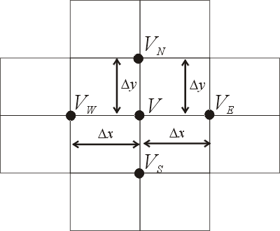
For the purposes of this discussion, we will use a rectangular grid to sample the voltage in two-dimensional space.  An example of this 2D sampling is shown in Figure 1.  The rectangular grid geometry is extremely easy to calculate and translate into a computer array of voltages.  There are actually many other types of sampling schemes for Laplace's equation that are optimized to certain types of problems.  Finite Element Method (FEM), for example, allows the engineer to sample space with non-uniform nodes; for FEM, regions of space that experience bigger changes in voltage receive denser samplings than regions of space with slow-varying voltages.  In this way, FEM places samples in space "where they do the most good", minimizing the computation time of very large problems.

Figure 1:  A uniform, rectangular network is used to sample Voltage in two-dimensional space.  From these discrete samples, we must estimate partial derivatives in x and y.

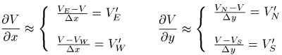
There are very few examples of electrostatic problems that can be solved using the analytic form of Laplace's equations.  Fortunately, we can recast Laplace's equation so that it may be solved by a computer.  To do this, we must find a way to approximate the second partial derivatives of voltage using our discrete samples in space.  Referring to Figure 1, if we want to approximate the first partial derivative of voltage at a point in space, we can construct an expression based on its neighboring voltages: V_N, V_S, V_E, and V_W (North, South, East, and West).  In fact, for the partial derivatives of voltage with respect to both x and y, there are two possible approximations we can use for each:

These approximations follow very logically from the definition of a partial derivative: they mark the change in voltage in the x or y direction, divided by the spatial increment that separates the samples.  Thus, we have two possible expressions for partial derivative with respect to x (which we will call V_E' and V_W') and two possible expressions for partial derivative with respect to y (which we will call V_N' and V_S').

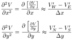
Now that we have approximations for the first partial derivatives, we can construct approximations for the second partial derivatives as well, based on the ideal that a second partial derivative is simply a "derivative of a derivative".  Thus, we can use the difference between V_E' and V_W' to estimate the second partial derivative in the x direction; we can use the difference between  V_N' and V_S' to estimate the second partial derivative in the y direction.  The equations for this are given below:

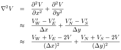
Now we have enough relationships to construct a discrete version of Laplace's equations in two dimensions.  Substituting these values into the definition of the Laplacian gives us:

It is this last term that, in the absence of charges in space, must be set equal to zero.

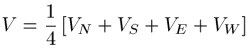
The most convenient choice of spatial increments is the case of Dx=Dy, which represents sampling on a square grid.  Under these circumstances, the discrete form of Laplace's equation becomes:

This equation is actually very simple: it states that a voltage at any particular point in uniformly sampled space must be the average of its nearest neighbors. So the discrete form of Laplace's equation is actually a 2D network of simple, interconnected averaging equations.  Therefore, an M x N grid of voltage samples will produce MN discrete equations that can be solved iteratively by a computer.  There is an online example in this tutorial that discusses how to solve the discrete Laplace equations as well as some Matlab code for solving and graphing the solutions to interesting 2D voltage calculations.

You do not really need to have complicated computer codes to solve Laplace's equation.  In fact, you can solve Laplace's equation very easily using only a spreadsheet!  Simply put this averaging formula in a grid of cells, surround the cells with boundary conditions, and then iterate the calculation until the voltage values appear to converge to a final answer.