Propagation Modeling
With Path Loss Exponent
At Geogia Tech
Stephen Gesualdo, Student,
Georgia Institute of Technology
Introduction
Propagation
models used today by many cellular companies need updating. These old models were designed for users in vehicles
traveling on roads, where there is low path loss. However, since the implementation of these
models indoor use of cell phones has increased heavily. Building penetration loss and shadowing
effects add considerable loss of power for indoor users. Updated propagation models accounting for
these losses are necessary in order to reduce outages for the indoor
consumer.
Propagation Model
This
section describes the theory behind the proposed propagation model. A discussion of the link budget equation,
path loss exponent, and antenna gain introduces an explanation of the
construction of the model.
Path Loss and Path Loss
Exponent
Path
loss is defined as the ratio between transmitted power and received power after
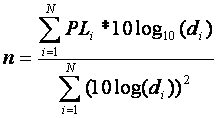
antenna gains and system losses have been controlled for. The link budget equation, given in Eq. 1,
shows this relationship in log form (dBm):
 (1)
(1)
where PT and PR
are in dBm, GT and GR are in dB, and PL is with respect
to 1 meter in freespace [1]. This path
loss includes distance dissipation and also losses due to shadowing and
penetration. A general path loss
exponent can be used in order to approximate path loss a region. Using the path loss exponent, n, path loss
would take on the form in Eq. 2:
 (2)
(2)
The path loss exponent is
specific to the propagation environment.
The value of n is 2 for free space and larger when obstructions are
present [2]. For practical use, n can be
found for an area if path loss measurements are taken at known distances using
the following equation:
 (3)
(3)
Measurements taken around the
Georgia Tech campus produce a path loss exponent of 3.4, which is consistent
with values measured in suburbs [1]. The
link budget equation with path loss exponent of 3.4 was used in the proposed
model, along with antenna directivity, discussed in the next section.
Antenna Gain
Antenna gain is determined by the shape of the
antenna. Antenna gain patterns are a
function of azimuth and elevation and have an associated half-power
bandwidth. Generally, the gain of an
antenna is higher when the directivity is more concentrated, i.e., the antenna
has a lower half-power bandwidth.
Antennas have an associated efficiency.
Gain can be described by:
 (4)
(4)
Where G is gain, φ is
azimuth, θ is elevation, and Ae is the effective aperture. Effective aperture is related to the size and
shape of the antenna and is also a function of azimuth and elevation [2].
For the proposed model, the shape of the antenna is
unknown. A general pattern for the gain
of the antenna can be deduced from data of power received around the
antenna. The directivity of the antenna
used in the model has a cos3/4(φ) dependency, with an
associated half-power bandwidth of 133o.
Modeling
To more effectively model wave propagation for indoor and
outdoor users, the proposed model uses the link budget equation in equation 1
with a path loss exponent. A path loss
exponent of 3.4 was obtained using recorded data from around the Georgia Tech
campus, including indoor measurements, from 3 different antenna sites. The data was plugged into Equation 3 to
obtain the value. The model employs a
gain pattern with a cos3/4(φ) dependency and a constant
multiplier of 25, which corresponds to peak gain. These values were obtained from measurements
around the Georgia Tech campus. The
receiver gain was not given. Using the
measured data and the wavelength corresponding to the given frequency of 850
MHz as 35.3 cm, a constant value of 7 dB is added to the model. A few other key concepts having to do with
location of the antennas are taken into account in the model.
The transmitting antennas are located on the tops of
buildings. The propagating waves can
travel over buildings and trees with relatively low loss. Directly behind buildings loss may be high
due to shadowing effects, but far behind the building loss may actually not be
severe due to propagation over the building. Thus path loss may not drop off with the path
loss exponent at far distances. In
addition, electromagnetic noise levels have been measured as high as -80 dBm at
industrial and inner city commercial sites [3].
For these reasons, the proposed model does not exceed -83 dBm.
The location of the antennas also effects power received at
small distances from the transmitter.
Measuring received power next to or inside of the building that carries
the transmitter antenna entails large penetration loss, and is also constrained
by the directivity of the transmitter with respect to elevation. For this reason, a level maximum level of -50
dBm is imposed on the model.
The transmitter gain is primarily focused “forward.” Antenna gain behind the antenna is dramatically
reduced; the power has been reflected to the front of the antenna. The proposed model has a maximum power of -70 dBm behind the antenna.
The model was coded using Matlab 7.0. The code for the model can be found in
Appendix A.
Results
The proposed model was tested for 4 different antennas at 3
different locations in the Georgia Tech campus.
The model was run using Matlab 7.0 and tested against measured data for
each of the 4 antennas. The average
error of the model was computed during the test in the form of standard
deviation and mean error. The model
obtained a standard deviation of 10.4 dB and a mean error of 2.6 dB. Figures 1 and 2 show the measured and modeled
data for antenna A.
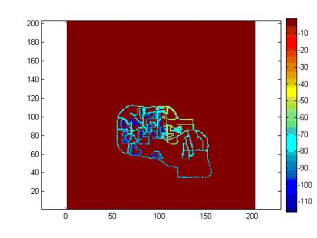
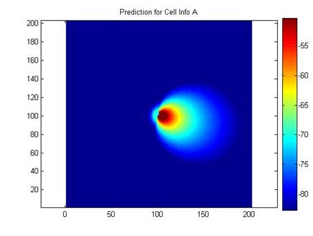
Fig. 1.
Measured power received from antenna A. Fig.
2. Modeled power received from antenna
A.
Error at site A is 9.99 dB standard deviation and 2.33 dB
mean. The model displays very symmetric
loss and does not account for building and road locations. However, the directivity of the model, as
opposed to a perfectly uniform path loss exponent, lowers the standard
deviation significantly. Results for
antennas B, C, and D can be found in Appendix B.
Conclusion
The proposed model computes received power strength with
moderate accuracy. The model provides a
very practical way for companies to predict signal strength in and around
buildings and around trees and roads.
However, the model does not use specific building locations. Immediate shadowing and penetration loss
effects are unaccounted for, thus users may still experience outages around
buildings if this model is relied upon too heavily. The model does work exceptionally well within
the half-power bandwidth in any environment.
The use of this model will decrease uncertainty compared to many current
models, and should save companies millions of dollars nationwide. There is still a large amount of revenue to
be captured along with a model that predicts penetration loss and shadowing
effects accurately.