Distinguishing between indoor/outdoor areas
The main approach taken with our propagation model was to first distinguish between indoor and outdoor areas and establish differing path loss exponents for those areas. To do so, an image mask of the buildings on campus was created using the IndoorMask.gif file shown in Figure 1. Because this image was not scaled to the size of the raster maps of received power provided by Springularizon, some image manipulation was required. To help fit the building mask image to the raster map, we first plotted a colormap of one set of received power data (Figure 2) and saved the colormap as an image file.
Figure 1. IndoorMask.gif showing the relative locations of buildings on the Georgia Tech Campus.
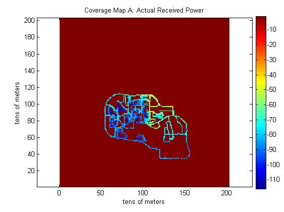
Figure 2. Color-coded map of received power data provided by Springularizon (this data set corresponds to Map A; see Documentation section for more information). The colorbar at left is in units of dB; areas in red (0 dB) denote locations where data was not taken.
We then imported both the building mask and the received power map into an image manipulation program such as Adobe Photoshop. The white background of the building mask was made transparent, allowing us to overlay the buildings mask over the power map and resize the mask as necessary to obtain the best fit.
Because the power map represents areas where data points were taken, we were able to discern the outline of several of the buildings and use them as reference points for the building image. For example, the Student Center parking deck is clearly visible as the L-shaped building in the lower left.
After the building mask was appropriately scaled, it was saved as a new black and white .gif file. However, we assumed that because the buildings provide a certain amount of interference to the surrounding outside areas, the path loss exponent in these areas would still be greater than the normal outdoor path loss. Therefore, two other outdoor "zones" around the indoor areas were defined as shown in Figure 3. These zones were defined more or less qualitatively based on patterns observed in the provided received power data sets.
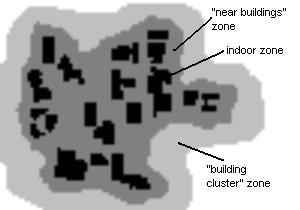
Figure 3. Final building mask as used in model, showing three different zones: indoor (black), near buildings (dark gray), and in a building cluster (light gray). The designation of zones was used to facilitate the assignment of different path loss exponents.
This three-tone building mask was imported into Matlab using the imread function and was used to identify indoor/surrounding areas.
Determining path loss exponents
The path loss exponents for each "zone" were determined through a mixture of statistical analysis, observation, and trial and error. For example, initial calculations using the equation
where where PL is path loss as determined by the link budget equation, yielded some preliminary path loss exponent values for inside and outside areas. Once path loss exponents were defined for all areas, the received power for each 10-m x 10-m map point was calculated with a direct application of the link budget equation, given by
Pr = ERP + PLref - PL(r)
where Pr is the received power,
ERP is the effective radiated power in dBm and is equal to transmitted power plus peak antenna gain,
PLref is the reference path loss, given by 20log(lambda/(4*pi)),
and PL(r) is additional path loss as a function of distance from base station r, given by 10*n*log(r).
Trial-and-error was then used. Based on the results from the predicted map generated, path loss exponents were further "tweaked" by small increments (0.1) in an iterative process of comparing the predicted power maps to the actual and altering the path loss exponents to yield better matching results.
During testing, it was found that in indoor zones farther away from the transmitter, path loss was actually too severe. To remedy this, each of the three "indoor" zones were further split into two different path loss exponents, one for a "close zone" near the transmitter and one for building areas that were farther away. The path loss exponent for the latter area was reduced slightly and again adjusted using trial and error.
It was also observed that a constant path loss exponent for the entire outdoors areas was not providing a large enough attenuation far away from the transmitter; in other words, the outdoor path loss exponent appeared to increase as distance away from the transmitted increased. This could representing general interference sources such as trees, uneven terrain, etc.
To model this, three outdoor zones were also defined: for distances up to 200 feet from the transmitter, the n used was 3, representing "urban area cellular radio"[1]. Beween 200 and 300 feet, we used a larger n, and for distances greater than 300 feet, we further increased n.
Table 1 summarizes the zones defined and the experimental path loss exponents used in the model.
| Zone | Distance from Base Station | Path Loss Exponent, n |
| Indoors (black) | < 250 meters | 4.5 |
| Near buildings (dark gray) | < 250 meters | 4.3 |
| Building cluster (light gray) | < 250 meters | 3.7 |
| Indoors | > 250 meters | 4.2 |
| Near buildings | > 250 meters | 4.0 |
| Building cluster | > 250 meters | 3.5 |
| Outdoors (near to station) | < 200 meters | 3 |
| Outdoors (midway from station) | > 200 and < 300 meters | 3.3 |
| Outdoors (far from station) | > 300 meters | 3.5 |
Table 1. Path loss exponents used in our model for various areas of campus and various distances away from the base station.
Further improvements
Information available to us that was not incorporated into the model included azimuth and transmit power of the antenna. Both of these would have helped give some directivity to the signal propagation.