WIMAXORBUST, INC.
Cellular Network Power Model
Using Large-Scale Path Loss and Terrain
Based Propagation Techniques
BRANDON CHONG, PROPAGATION
ENGINEER, DES Group
MODEL DESIGN: ANTENNA RADIATION PATTERN
MODEL DESIGN: LINE-OF-SIGHT ISSUES
MODEL DESIGN: LINK BUDGET
EQUATION
MODEL DESIGN: EMPIRICAL FITTING
WITH MEASURED DATA
Unfortunately in modern wireless communications, signal strength is no longer simply a function of how the distance from the transmitter. With obstacles such as hills and buildings being constructed at a growing rate, many other factors begin to affect the received signal strength such as signal diffraction, scattering, and reflection. Furthermore, some of these factors become even more complex when discussing multiple paths to the receiver and the phase changes of the signal in taking these paths. Older propagation models are becoming outdated and Wimaxorbust has consulted Double-E Students (DES) group at the Georgia Institute of Technology to design a propagation model for their cellular network that operates at 1920 MHz.
The model design
serves to accurately predict received signal strength in areas of around 1000
square kilometers (a few
MODEL DESIGN: ANTENNA RADIATION PATTERN
One large factor affecting the signal strength received at a location is the orientation of the antenna transmitting the power to the receiver. A typical cellular base station antenna has a 120º half-power bandwidth centered at its angle in azimuth (the direction it is facing). This means if you are at a location 60º from where the antenna faces you will only receive about one half of the peak transmitted power, the further away you are from the antenna's direction the less the signal strength. Most cellular base station antennas have a front-to-back ratio ranging from 25dB to 45dB [1]. The value of 30dB is chosen in the model design for the front-to-back gain ratio.
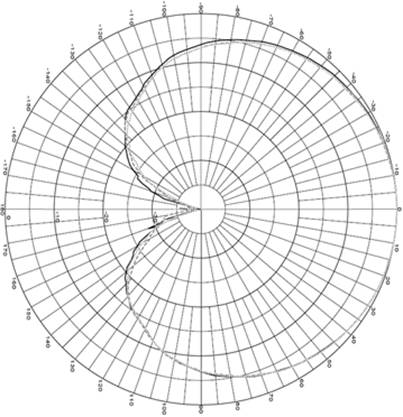
Figure 1. Antenna gain pattern for a 120º half-power bandwidth directional antenna (in dB) [2].
Figure 1 shows a typical antenna pattern that would be similar to that of a cellular base station's antenna if it's angle in azimuth was 0º, notice that 60º from the azimuth angle the power has dropped by -3dB. This gives three conditions for modeling the cellular base station's antenna radiation:
- That the gain is 0dB in the direction the antenna faces.
- That the gain 60º from the direction the antenna faces is -3dB.
- That the gain behind the antenna (or 180º) from the direction the antenna faces is -30dB.
A mathematical model that would satisfy all three of these conditions is shown in equation 1.
![]() (linear gain)
(Equation. 1)
(linear gain)
(Equation. 1)
Where
delta_angle is the difference between from the antenna's orientation in azimuth
and the angle of the path to the receiver in azimuth, normalized so it is
positive and between 0º and 180º. a_1 = 0.246335667 and a_2 = 20.6, which are
attenuation constants determined empirically from this spreadsheet. A plot
of this mathematical model of the antenna's gain pattern is shown in Figure 2.
Figure 2. Modeled antenna gain pattern (linear gain).
The use of this mathematical model created loss maps such as the one shown in Figure 3. Where the location of the transmitter and its direction are shown.
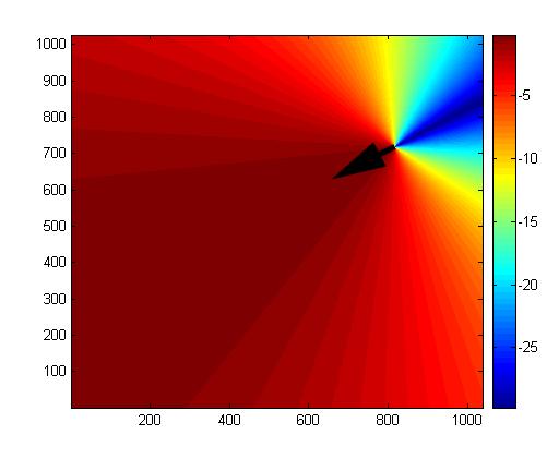
Figure 3. Calculated loss map from base station orientation.
The following MATLAB functions were used to create a map of the loss from the antenna orientation:
find_angle calculates the angle in azimuth to the receiver from the transmitter.
directional_loss subtracts the angle of the transmitter from the angle of the path to the receiver, normalizes it, and returns the loss from the peak gain in dB.
directional_loss_map uses directional_loss at every point on the map to create a map of loss from transmitter orientation.
MODEL DESIGN: LINE-OF-SIGHT ISSUES
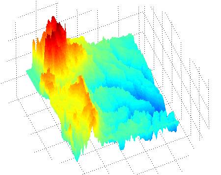
Another factor of significant loss of signal strength is blockage. A receiver that has direct line-of-sight path to the transmitter has a much higher signal strength than one that is obstructed by a hill or a building. Thus the use of the terrain maps provided by Wimaxorbust come into play. A mathematical algorithm using the terrain map was created to determine if a direct line-of-sight path existed between the transmitter and receiver. This algorithm consisted of find a slope by dividing the difference of the height of the radiating antenna and the receiving antenna by the distance between them, and then tracing a straight line path between the antennas, regularly checking if the height of the terrain was greater than that of the slope, and therefore causing a blocked signal. The simplest way to model the effects of this blockage was to insert an extra blockage loss constant of -6.31 dB(empirically determined), whenever a signal was blocked. This is done mathematically by multiplying the blockage map by -6.31 to create a map of the blockage loss.
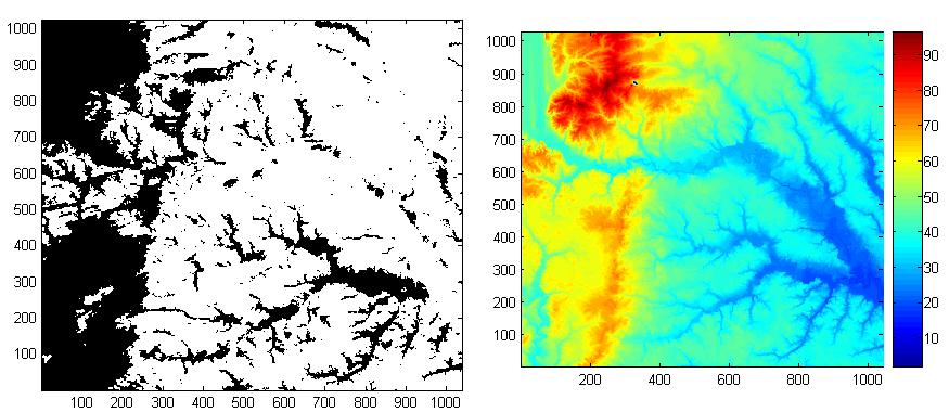
Figure 4. Comparison of terrain map and blockage map.
Figure 4 shows a side-by-side comparison of a generated blockage map and a terrain map. The blockage map on the left shows the blocked areas in black and the areas with a direct line-of-sight in white. A quick examination shows that the blockage map is accurate.
The following MATLAB functions were used to create a map of the line-of-sight blockage:
blocked_path checks if the path from transmitter to a receiver at a certain location is blocked.
blocked_map uses blocked_path to generate a map.
MODEL DESIGN: LINK
BUDGET EQUATION
The Link Budget Path Loss equation is a well known equation that allows calculation of received power given the values of its other variables. The equation, shown in Equation 2, puts together all the transmitter characteristcs and all possible losses due to path loss or any losses in the system.
Link Budget Equation
![]() (in dBm)
(Equation. 2)
(in dBm)
(Equation. 2)
Where
PR is the received power, PT is the transmitted power, GT
is the gain of the transmitting antenna, GR is the gain of the
receiving antenna, ![]() is the operating
wavelength, n is the path loss exponent, r is the distance between transmitted
and receiver, and L is system loss not related to propagation. In the model
designed for Wimaxorbust, Equation 2 is used in its entirety, adding the loss
from the antenna gain pattern and a blocked direct line-of-sight to obtain a
more accurate value for received power. Wimaxorbust specifies the effective
isotropic radiated power, which is the transmitted power and the gain of the
transmitting antenna. The value used for the path loss exponent is
2.78(determined empirically). Wimaxorbust also does not specify the gain on the
receiving antenna used for their measurement maps, so it is assumed to be 0dB
for now. The system loss term is also assumed to be 0dB. This final revised
Link Budget equation allows the use of the designed model to predict signal
strength over the mapped area.
is the operating
wavelength, n is the path loss exponent, r is the distance between transmitted
and receiver, and L is system loss not related to propagation. In the model
designed for Wimaxorbust, Equation 2 is used in its entirety, adding the loss
from the antenna gain pattern and a blocked direct line-of-sight to obtain a
more accurate value for received power. Wimaxorbust specifies the effective
isotropic radiated power, which is the transmitted power and the gain of the
transmitting antenna. The value used for the path loss exponent is
2.78(determined empirically). Wimaxorbust also does not specify the gain on the
receiving antenna used for their measurement maps, so it is assumed to be 0dB
for now. The system loss term is also assumed to be 0dB. This final revised
Link Budget equation allows the use of the designed model to predict signal
strength over the mapped area.
Revised Link Budget Equation
![]() (in dBm) (Equation.
3)
(in dBm) (Equation.
3)
Where the variables are the same as in Equation 2, the EIRP is the effective isotropic radiated power specified by Wimaxorbust, the AntennaDirectionalLosses are the losses from antenna orientation calculated in the previous Antenna Radiation Pattern section, and the BlockageLoss is the blockage loss from the Line-of-Sight Issues section.
This MATLAB function takes in a variable with the terrain map, antenna direction loss map, blockage loss map, antenna characteristics, and returns a predicted received power map:
MODEL DESIGN: EMPIRICAL
FITTING WITH MEASURED DATA
After the model is created, it is tuned with Wimaxorbust's measured received power maps to further increase the accuracy. Since all of the values are in maps, or essentially matrices, the model is tuned using MATLAB. Since the antenna directional loss pattern exhibits the desired characteristics, the received power maps are used to find the optimum blockage loss constant, path loss exponent, and any extra loss that would make the model more accurate. This was done using a function that predicts maps with different blockage loss constants, path loss exponents, and extra constants, then compares the predicted maps with Wimaxorbusts measured maps to find an average mean error and average standard deviation of error. The function then plots mean errors, and standard deviations against the changing variables as shown in Figure 5.
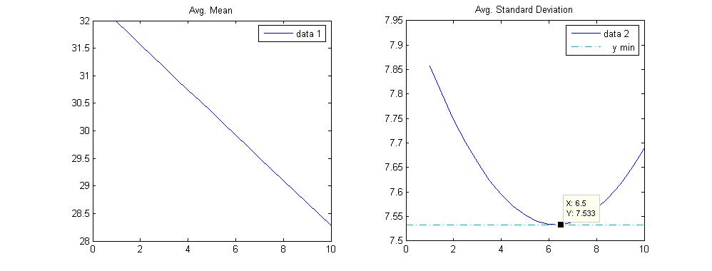
Figure 5. Plot of mean error and standard deviation v. blockage loss constant as it goes from 0 to 10.
The optimum values for each variable can simple be determined by finding its value where the standard deviation is at a minimum. After the optimum blockage loss constant, and free space path loss exponent is determined. The average mean error is nullified by adding an extra constant that makes the average mean error small as possible.
The optimum values are calculated using this method to be -6.31 for the blockage loss constant, and 2.78 for the path loss exponent. This value for the path loss exponent corresponds with an area that has more loss than free space (path loss exponent of 2) and less loss than an urban area (path loss exponent of 2.7 to 3.5) [3]. This reinforces the accuracy of the model since the area modeled is based on terrain, which is usually not as cluttered as a city crowded with buildings, yet more cluttered than an ideal free space. The extra constant added determined to be +1.06dB which can easily be contributed to a combination of the receiver gain and system loss, previously assumed to be zero.
The following MATLAB functions were used to empirically fit the data:
model_prop predicts signal strength maps with different variables, compares with measured data, then plots variables v. mean and standard deviation.
CompareMaps is used to compare two received power maps and return the mean error and standard deviation.
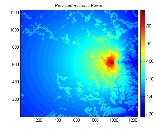
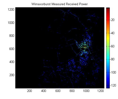
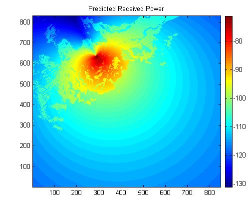
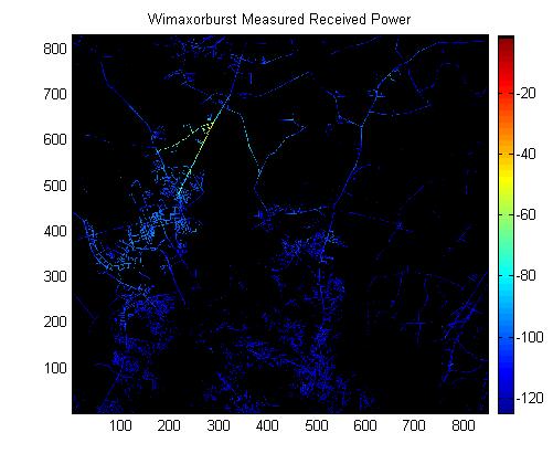
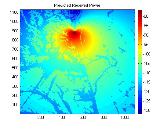
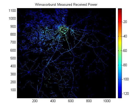
The predicted signal power map and the Wimaxorbust measured signal power map are shown for Cellular Base Stations A, B, C, and D. The black areas on the Wimaxorbust maps are either unmeasured or measured with signal strength too low to record. Standard deviation and mean error is also given for each station's comparison.
Wimaxorbust Cellular Base Station A
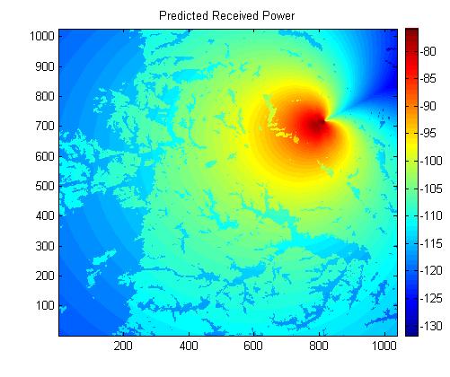
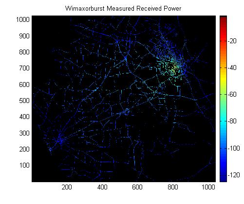
Mean Error of -2.33 dB, Standard Deviation of 7.28 dB
Wimaxorbust Cellular Base Station B
Mean Error of +2.52 dB, Standard Deviation of 7.01 dB
Wimaxorbust Cellular Base Station C
Mean Error of +1.68 dB, Standard Deviation of 6.80 dB
Wimaxorbust Cellular Base Station D
Mean Error of -1.84 dB, Standard Deviation of 7.55 dB
Average Error of (Mean = 2.1 dB, Sigma = 7.2 dB) for 4 site(s)
The geometrical theory of diffraction takes into consideration a few basic principles. One is Fermat's Principle that light takes that shortest path, and will even refract around corners to arrive at a certain point. GTD also says that the front of a moving wave can be treated as a source creating more waves. This moving plane reaches the edge of an obstruction and then begins emitting waves into the area that is not in line-of-sight of the incoming wave. The boundary where the waves are in line-of-sight and the boundary where they are not is called the shadow boundary. The magnitude of the refracted waves is related to a Fresnel function centered at each shadow boundary.
The designed model does not use any diffraction theory in the design, but takes diffraction into account by using an empirical method to design it with the help of Wimaxorbusts measured signal strength maps. By changing some of the variables within the Link Budget equation, the effects of other propagation methods are felt when those variables are optimized to the measured signal strength maps.
The practicality of the model is that the standard deviation is around 7.2dB and it is not ready to be used to model a national cellular network. Although this model would be helpful in the placement of cellular base stations, its signal strength predictions become less accurate with more obstructions. The model fails to use propagation methods such as scattering, diffraction, and reflection and would likely have a higher error in many urban areas where these obstructions are numerous and scattering, diffraction, and reflection may be the main methods of propagation.
If the use of the model became more widespread, it would have to be empirically fitted for different regions, and would not be very economical.
[1]
Best, Steven R. Antenna Performance and
Design Considerations for Optimum
Coverage in
Wireless Communication Systems. Antenna Performance Considerations. pp. 1-7.
[2]"120º Sector Antenna Pattern." http://www.wlanantennas.com/catalog/product_info.php?products_id=48&osCsid=a7f77e62c7d960369567810e4701e
349.
[3] Rappaport, Theodore S. Wireless Communications Principle and Practice. 2nd Edition.