Microwave Radio Terrain Diffraction Modeling

II. Model Used

    - Part 2

III. Testing / Results

IV. References

1. Development

a) At first, it was assumed that the antenna was omnidirectional and the map operated as free space.  Distances were calculated between each point as being in 2-D space.  This was used to set up base code and to see how much error is possible in a model based solely on radius and frequency loss using the formula map(i,j) = BSpower - (20 * log10(4 * pi / lambda))  - 20 * log10(dist).   This turned out to be a mean error of over 32.3 dB.

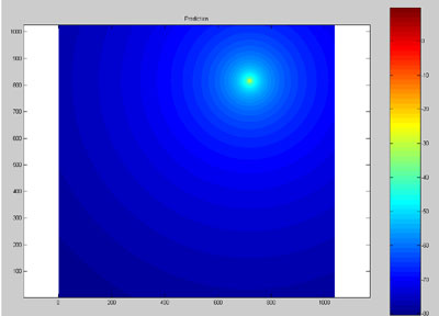
Omnidirectional Antenna / Free Space / 2-D Model.

b) Next, elevation information was taken into account when calculating the distance between the base station and each point. This only cut down the mean error by about 1dB, but was intended to set up diffraction information for the future.

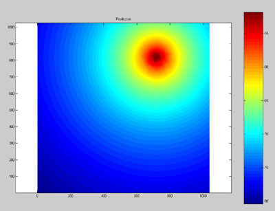
Omnidirectional Antenna / Free Space / 3-D Model.

c) At this point, the error maps showed that the largest source of error was coming from "behind" the antenna.  The next step was to model the antenna as a directional antenna with 120 degrees of spread.  In order to take advantage of this, two path loss exponents were set up, one for the front of the antenna and one for points lying behind it.  This model produced a mean error of 3.25dB and a standard deviation of 11.96dB.

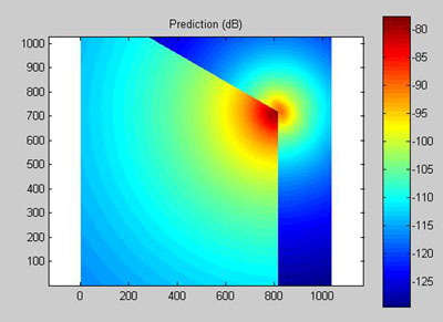
Directional Antenna / Path loss / 3-D Model.

d) At this point, the largest error still was coming from the directionality of the antenna.  The side lobes were far underestimated, so a three-stage model was used instead of the current two-stage model.  This slightly raised the mean error to 3.3, but drastically lowered the standard deviation to 7.4.  The code used to generate this can be found in the file processdata.m

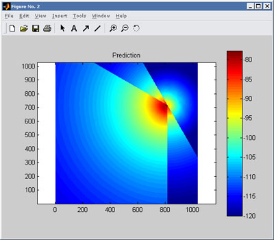
Directional Antenna / Path loss / 3-D Model.

e) Finally, elevation changes that created shadows became the most significant source of error in the model.  Continue to part two of the development for information on this