SARSAT Rescue

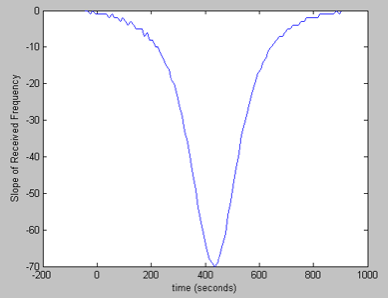Figure 1. The first derivative of the received frequency. The location of the minimum indicates the time of closest approach (TCA) and the magnitude is relative to the distance from the EPIRB to the satellite. Specifically, the closer the two are, the greater in magnitude the TCA slope will be.
Figure 2. Using the simulate and match method, we could find a simulated curve that matches the measure. The blue line is the measure value, and the two red lines are example guesses. The correct guess would align perfectly along the middle section of the blue curve.

In Figure 1, a plot of the received signal frequency, which is a decreasing function with horizontal asymptotes located where the minimum and maximum Doppler shifts occur. The relative velocity of the satellite to the beacon causes a frequency shift in the signal received by the satellite. When the satellite is far away from the beacon, the frequency shifts are at a maximum, forming horizontal asymptotes. As the angle between the satellite and the beacon decreases, the relative velocity of the two also decreases. This reduces the Doppler effect measured at the satellite. When the latitude of the satellite and the beacon equals, there is no frequency shift. After the satellite’s latitude passes the EPIRB’s latitude, a negative frequency shift occurs.

It may be presumed that the satellite is at the same latitude as the EPIRB when the satellite receives a signal having a frequency of 406 MHz. However, due to perturbations in the clocks of the satellite and EPIRB, we cannot assume that the EPIRB is transmitting at exactly 406 MHz, or that the satellite is reading exactly 406 MHz. Because of this error, we measured the time when the received signal’s frequency is exactly halfway between the two asymptotes resulting in a frequency of 406.000065 MHz.

To find the longitude of the EPIRB, we need to calculate the distance between the EPIRB and the satellite (the satellite is on the 76°W longitude line) at an altitude of 850 km. To find the longitude, we used simulation match method. This involves generating numerous plots using an increasing longitude and comparing each plot to the plot generated from the received data. We then chose the plot whose slope was closest to the data plot’s slope. We show a few simulated guesses in Figure 2. Using this method, we were able to narrow the latitude down to 25.4445°N. This places the EPIRB about half way between the coast of Miami, FL and the island Bimini.

The following code implements the technique described above to calculate the longitude and latitude of the EPIRB.

• plotpath3d.m creates a vector of 3-dimensional distances between two points. Then creates a velocity by deriving the samples. It returns the slope of the velocity curve at the TCA.
• myslope.m calculate the slope of a curve by taking a center index and two offsets from the center and calculates the rise over run.
• project1.m uses plotpath3d to find the curve with the minimal difference in slope of the simulated and measure velocities at the TCA. It iteratively refines its guesses until a threshold match is found.

Questions Section

1. Are there any ambiguities in your technique? How might these be addressed?
   Yes, these ambiguities would stem from the simulated matching method used to calculate the longitude of the EPIRB. We could reduce the amount of error encountered with this method by taking measurements in the field and correcting the received data based on our real measurements.
2. Can you place a confidence interval on your position estimate?
   The level of error in our calculations mostly comes from the simulated match method. This method can iterate into almost infinite precision (we stopped at 10^-6 degrees) but the input data was our limitation on accuracy. Also, we have no model for the noise of the input readings. If we assume perfect readings and a smooth, constant-radius spherical Earth, then our method would be accurate to the micrometer. As it is now, we believe our method to be accurate to within 50 km in the longitudinal direction.

   The latitude accuracy is limited by our clock resolution. At ten samples per second, the satellite crosses 0.00581 degrees of its path around Earth, which relates to 37.2 km of ambiguity without interpolation.

3. How might a receiver measure carrier frequency?
   
   
   Figure 3. Illustration of the beatnote magnitude for two additive sinusoids, one at 440 Hz, and the second at 442.5 Hz, forming a 2.5 Hz beatnote.
   Measuring frequencies accurately, is a major industry in laboratory equipment. Since we know, within a close proximity, the frequency we wish to detect, we can add our key frequency (406 MHz) to our received signal and measure the "beat notes" that form. A beat node, often used for guitar tuning, forms when two close frequencies add together. The phasing in and out of the two additive signals creates a varying magnitude of the signal (easily measured with an RC circuit) with a frequency of the difference between the received frequency and the key frequency.
   Once we generate the beatnote frequency, we can measure it using various methods. A cheap zero-crossing counter may work well, if the sampling is slow enough that the noise power will not create spurious crossings. Simply measure the time between crossings and it is inversely proportional to your frequency offset. If the offset decreases between measurements, then the frequencies are closer together and most likely the received frequency is higher than the key frequency. When the beatnote frequency offset increases, then the received frequency can be assumed to be lower than the key frequency.