The carrier frequency for our communication link with the Epsilon Eridani Space Probe (EESP) will be 270 GHz. Such a high frequency will allow us get very high gain using reasonably sized antennas. However, 270 GHz has a high atmospheric attenuation of about 6 dB/km. To overcome this crippling loss, we propose the use of a space based repeater satellite (SBRS).

There are two main problems with using a SBRS that orbits the earth. The first problem is the relative high speed of the SBRS as it orbits the earth. This presents a problem in terms of varying Doppler shift and keeping it pointed in the right direction. An SBRS that orbits the earth will also have its view of the probe blocked by the earth a high percentage of the time. Blocking for a high percentage of the time is unacceptable since we will have no means of acknowledgment of receipt due to the long transit time. Since having our SBRS in an orbit around the earth is less than ideal, we propose placing it on or in a small orbit about Lagrange Point 2 (L2) as seen in the animation to the right. This will allow us to be outside of the earth's atmosphere and magnetic field, to have a vantage point that is more stable than on the earth or in an orbit around the earth, and to maintain a very low system noise temperature. To protect the SBRS from the Sun's radiation, we will require a large solar shield similar to what NASA will use for their WEBB IR telescope which will be launched to the same orbit as early as 2014. ^[1]

The communication hardware for the SBRS and the EESP will be similar. Both will have a dish that is 40m in diameter. The dish could either be packed up, and unfurled in space, or launched in sections and assembled in space. The dishes would have to be manufactured with very tight tolerances as the standard deviation of the surface roughness could not exceed 1.388x10^-4m. With a dish of this size we can achieve a gain of about 100dB. The half-power beam width in terms of degrees would be extremely narrow at 1.53x10^-3°. Due to the extreme distance, the beam will be over 2.6x10¹²m wide at the target.

The SBRS will also need a second communication link with the earth base station. Because the distance between the SBRS and Earth is much smaller than that between SBRS and EESP a more traditonal satellite communication scheme can be used. The carrier frequency will 2.4GHz. The Earth station will use a 9m dish and the SBRS will use a 6m dish. The Earth station should be at a high latitude to allow longer possible SBRS viewing times. The increased attenuation due to the increased path distance through the atmosphere will be negligible.

References

1. The James Webb Space Telescope

Full-duplex transceivers will be used for communication with the probe. The transceivers used for the SBRS and EESP are of identical design. The system is primarily digital, with only an analog RF front end. A radiation-hardened FPGA lies directly behind the DAC and ADC of the front end as shown in the schematic. The front end employs variable oscillators to adjust for doppler shift on the receive side. Thus, it receives at 237.6 GHz when at coast speed and always transmits at 270 GHz as long as the speed difference between the SBRS and probe gives a doppler shift greater than ~2 kHz.

On the receive side, the FPGA performs downconversion of the 25 MHz IF to baseband, symbol recovery, and decoding. The transmit side is exactly the opposite operation - encoding with LDPC, BPSK modulation, and upconversion to a 25 MHz IF.

The earth/SBRS link uses essentially the same architecture as the EESP/SBRS link but at different frequencies and bit rates. The transmit side uses a 2.5 GHz carrier and the receive side a 2.4 GHz carrier.

Figure 1. EESP Transceiver (left) and SBRS Transceiver (right) block diagrams

After the data leaves the FPGA, it continues on to the central control unit on the probe where it may be stored in RAM or on a hard disk for buffering before transmission. Storage and buffering are absolutely necessary due to the very low 333 Hz bit rate of the transit receive system. The same operation happens at the SBRS where the received data may be buffered before being transmitted to earth.

Due to the very low received power on the SBRS to EESP link, BPSK modulation will be used. BPSK is ideal in this scenario because it is simple and will lead to a lower BER. The SBRS to Earth link will also use BPSK modulation to keep both legs of transmission similar. However, since the distance between the SBRS and is much smaller than that between SBRS and EESP, a more traditonal satellite communication scheme can be used. Both links will also use the same Raised Cosine pulse shape.

SBRS to EESP Link Modulation BPSK Carrier Frequency 270GHz Raised Cosine Pulse Rolloff 0.4 Bandwidth 1kHz IF 25MHz Coding 1/2 rate LDPC Symbol Period 1.5x10-3s Bit Rate 333.3 bps	SBRS to Earth Link Modulation BPSK Carrier Frequency 2.4GHz Raised Cosine Pulse Rolloff 0.4 Bandwidth 1MHz IF 25MHz Coding 1/2 rate LDPC Symbol Period 12x10-7s Bit Rate 4.17x105 bps
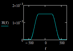
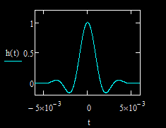
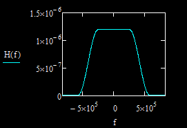
SBRS to EESP link baseband SBRS to EESP link pulse shape	SBRS to Earth link baseband 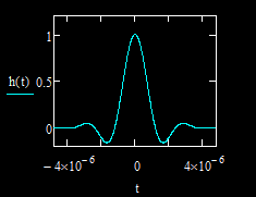SBRS to Earth link pulse shape

The received signal must allow reconstruction of excellent pictures of Epsilon Eridani. The communication channel will be subject to noise, and thus, errors may be introduced during transmission from the satellite. Therfore an error detection and correction technique must be impemented in the system.

Low Density Parity Check (LDPC) codes, which approach Shannon's capacity, were chosen. Since 2001, it has been possible to achieve a BER smaller than 10^-5 with an SNR of 0.0045 dB and a 1/2 rate code.

LDPC codes can be represented by a parity check sparse matrix or a Tanner Graph. A "1" in the i^th line and j^th column means that variable node j will be connected to check node i in the Tanner graph. Several algorithms exist to decode LDPC codes, and the belief propagation one with 10 iterations will be used.

Here is an example of a (not so sparse but good to understand the algorithm) parity check matrix H and its Tanner graph:

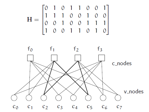
Let the source codeword be [1 0 0 1 0 1 0 1]. The check word, calculated by multiplying our codeword by H transpose, is [0 0 0 0]. Assume that, during transmission, one bit changed and the received codeword became [1 1 0 1 0 1 0 1].

The decoding algorithm starts here, where each variable node c_i first sends its bit to each check node f_j:

• f₀ node will receive 1 1 0 1 bits from c₁, c₃, c₄ and c₇ accordingly.
• f₁ node will receive 1 1 0 1 bits.
• f₂ node will receive 0 1 0 1 bits.
• f₃ node will receive 1 1 0 0 bits.

Then, every check node, f_j, calculates a response to every connected variable node c_i. The response message contains the bit that f_j believes to be the correct one for this variable node c_i assuming that the other variable nodes connected to f_j are correct. Here are the responses of check node 0 to its variables nodes 1, 3, 4, and 7:

• Response to c₁: if c₃ = 1, c₄ = 0 and c₇ = 1 are correct, then c₁ has to be 0 (the modulo 2 sum of them has to be the first bit of the check word = 0).
• Response to c₃: if c₁ = 1, c₄ = 0 and c₇ = 1 are correct, then c₃ has to be 0 (the modulo 2 sum of them has to be the second bit of the check word = 0).
• Response to c₄: if c₁ = 1, c₃ = 1 and c₇ = 1 are correct, then c₄ has to be 1 (the modulo 2 sum of them has to be the third bit of the check word = 0).
• Response to c₇: if c₁ = 1, c₃ = 1 and c₄ = 0 are correct, then c₇ has to be 0 (the modulo 2 sum of them has to be the fourth bit of the check word = 0).

After all check nodes are processed, each variable node has the following set of bits:

• c₀: 0 from f₁, 1 from f₃, 1 from originally received codeword.
• c₁: 0 from f₀, 0 from f₁, 1 from originally received codeword.
• c₂: 1 from f₁, 0 from f₂, 0 from originally received codeword.
• c₃: 0 from f₀, 1 from f₃, 1 from originally received codeword.
• c₄: 1 from f₀, 0 from f₃, 0 from originally received codeword.
• c₅: 0 from f₁, 1 from f₂, 1 from originally received codeword.
• c₆: 0 from f₂, 0 from f₃, 0 from originally received codeword.
• c₇: 1 from f₀, 1 from f₂, 1 from originally received codeword.

Then using the voting for each bit (i.e. which bit has more 'votes' in the above table out of three cases) creates a new codeword: [1 0 0 1 0 1 0 1]. Here, the right codeword is found after the first iteration because it is a simple example, but in many cases more iterations would have been needed.