Indoor/Outdoor Propagation Modeling on Georgia Tech Campus

James Armstrong - gtg604k@mail.gatech.edu

Propagation Model

In order to determine the received power values of the 4 unknown antenna maps, path loss exponents had to be determined. The received power maps from the 4 known antennas were utilized during this process. Although the task seemed relatively simple at first, it eventually became complicated by the fact that the path loss inside and outside the azimuth were calculated with difference of 20dB.

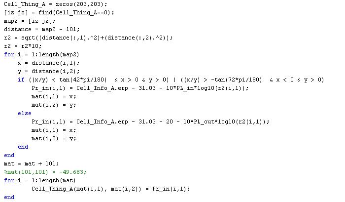
In order to determine the received power values inside the azimuth, basic trigonometric functions had to be recalled and applied within a matrix. The location of the received power values inside the azimuth could be referenced to by centering the task on the location of the azimuth. Adding and subtracting 60 degrees from provided azimuth value produced an area within the matrix which included the power values. Since each azimuth was different for each antenna, several scripts needed to be written in order to determine the path loss values within and outside of the azimuth. The following includes the code used to determine the coordinates inside and outside of the azimuth:

Along with determining the coordinates and received power values inside and outside of the matrix, the distance for each point needed to be determined. Simply iterating through each coordinate with the basic formula:

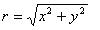
the distance from each point to the transmitter was able to be determined. Now that every value needed to calculate the Path Loss was determined, the path loss, and path loss exponent, inside and outside the azimuth was calculated, using the following code:

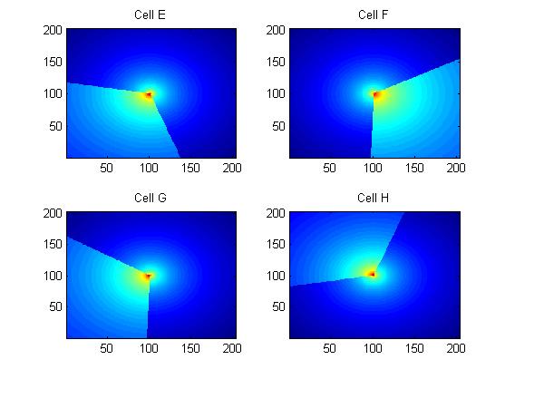
Now that every Path loss exponent was determined, the process in predicting the received power maps could start. In order to start this process, however, the azimuth-determining code would need to be used again. However, this time, an empty matrix was used, as opposed to one including the different power values. The code used for these maps is displayed below:

Also displayed was the code used in order to create a 203 by 203 matrix full of predicted received power values for the other 4 maps.

Below are the path loss exponents calculated, for both inside and outside the azimuth, for each map:

Table with Path Loss Exponents

The Path Loss values for Maps E, F, G, and H were determined by averaging values determined from maps A, B, C, and D based on their location, relative to the azimuth on the unknown map. Displayed below are the 4 predicted maps: