| |
| Introduction |
The propagation model I used to predict the path loss for the locations where data had been previously measured was a modified Cost231 Hata model [1]. I used the Path Loss Exponent model [2] for the unmeasured locations.
The modifications to the Cost231 Hata model were quite extensive. Over 25 correction factors were used to account for differences in terrain, directionality of the transmitting antenna, and other losses.
|
| |
Cost231 Hata Model
|
| The Cost231 Hata path loss model is defined in [1] by the equation: |

|
| |
where |
fc = carrier frequency (MHz)
|
| |
|
hb = base transmitter height (m) |
| |
|
d = distance (km) |
| |
|
c = correction factor |
| |
This model was specifically designed for carrier frequencies above 1600 Mhz. Modifications were going to be needed to make it fit the project. A heuristic approach was used to determine which parameters needed to be changed. |
| |
Path Loss Exponent Model |
| The Path Loss Exponent model is defined in [2] by the equation: |
 |
| |
where |
n = path loss exponent |
| |
|
d = distance (m) |
| |
|
Xs = Gaussian random variable |
| |
The Gaussian random variable has a mean of 0 and a standard deviation of 1 and n is defined as: |
 |
| |
where |
di = distance at each measured location (m) |
| |
|
PLi = path loss at each measured location |
| |
PLi can be found by using Friis Free Space equation. This can be calculated by using the power received at each location and the equation: |
 |
| |
The meaning of these parameters can be found in the theory section. |
| |
This model was used for the unmeasured locations because my model for the measured locations is dependent on proper classification of what region the receiver is in. This information would be difficult to determine for the unmeasured locations. |
| |
McAllister Dodger Model |
The final model used for the measured locations, from here known as the McAllister Dodger model, is: |
 |
| |
where |
fc = carrier frequency (Hz) |
| |
|
hb = base transmitter height (m) |
| |
|
d = distance (m) |
| |
|
c = correction factor |
| |
Changing the model to use the natural logarithm and different units for fc and d allowed the model to have a greater sensitivity to parameter changes. This allowed the choice of correction factors to be more precise. |
| |
As the height of the base transmitter was unknown, this value was chosen such that it reduced the standard deviation by the most amount. The correction factors were also chosen in a way to reduce the standard deviation. |
| |
| Terrain Classification |
The terrain is classified using 8 different regions to account for locations that are indoor or outdoor or somewhere in between. These regions were found by grouping the measured data by received power strength.
These regions are highly dependent on the actual data obtained and the direction the antenna is facing. Some modifications to the regions of the prediction sites were done to account for these issues. The region maps for cell sites A through D are shown below. Click the image for a larger picture.
|
| |
| |
| Directionality |
Directionality of the antenna is found by dividing the map into three directionality regions and creating a separate model for each using the two models discussed above.
The first region is found by adding ± 58° from the azimuth to account of the beamwidth of the transmitting antenna. The second region is found by adding ± 30° more to account for the side lobes. The last region is defined as everything else.
An example picture of this process is shown below. These regions were found from using cell site A, which is facing 102° azimuth .
|
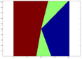 |
Cell Site A |
|
|
| Matlab Code |
The code I used was slightly different for the three base transmitter locations because of the correction factors and directions of the transmitting antenna. The Matlab code for the three models I used for the three locations are below. |
|
| The code has been commented to explain the purpose of each code segment. |
| |