There are many different theoretical as well as empirical models used for long range microwave propagation over various terrains. The theoretical methods provide reasonable results on paper when all interference is defined to be simple knife edges and screens of known dimensions. Unfortunately, when making measurements in the field, the crude but necessary approximations of terrain cause the theoretical results to vary greatly with the actual measurements. Similarly, empirical formulas can be made for a specific region or specific type of terrain, but when applied to somewhere other than where it was derived, the predicted results will no longer match the actual measurements. Therefore, it is only with a combination of both theoretical calculations and empirical formulas that a general microwave propagation algorithm can be created.
The best approach to creating a model is to start with the most basic concepts and build up from there increasing the accuracy as the model becomes more complicated. In its most simple form, large scale propagation modeling is given by the following equation. Note that this logarithmic equation applies to free space.
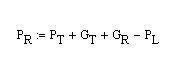
For this model, the power transmitted, PT, and the antenna gains, GT and GR, are combined into the effective isotropic radiated power (EIRP) since the specific parameters are unknown.
The remaining term is path loss, PL and can be defined by the following equation:
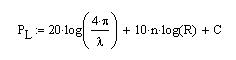
λ:propagating
wavelength
n:path loss exponent
C:correction factor
The path loss exponent is calculated empirically using the 4 test regions. Since the path loss experiment is calculated this way, it will be rather general and can be applied to a wide range of terrains.

The distance R in all of the preceding formulas is the distance between the transmitter antenna and where the measurement was made and is calculated simply by using the quadratic equation. It accounts for the distance in the displacement in the x and y direction and also the altitude at which the transmitter and receiver reside.
The correction factor changes the result accounting for any excess
loss or gain that was not considered in the theoretical calculations and was
determined empirically with the four sample regions. When first estimating the received power using
Equation 2 without C, the results had a relatively low standard deviation but a
significantly large mean for each region.
By setting C equal to the negative average of the means, they
were
essentially eliminated thus greatly improving the accuracy. The
only remaining method to improve the quality of the model is to
directly incorporate diffraction.