|
Our
propagation modeling technology is based on
incorporating terrain diffraction, clutter losses and
distance path loss. Although we have the capability to
incorporate all three of these losses in our model, many
of these loss models are computationally expensive and
are not necessary in all cases. For example, if the
signal was not propagating through an area with great
terrain variations, the return on investment of
computing power is minimal.
Variations in terrain can play a significant role in
signal propagation. Many times terrain can block the
line of sight between the sending antenna and the
receiving antenna. In this case, the signal that is
received is only the signal that was diffracted from the
terrain. In the interest of simplifying the diffraction
calculations, terrain can be modeled as a perfect
electric conductor (PEC) edge, as shown in Figure 1, and
then approximate the effects of diffraction using the Sommerfield
solution for a PEC edge.
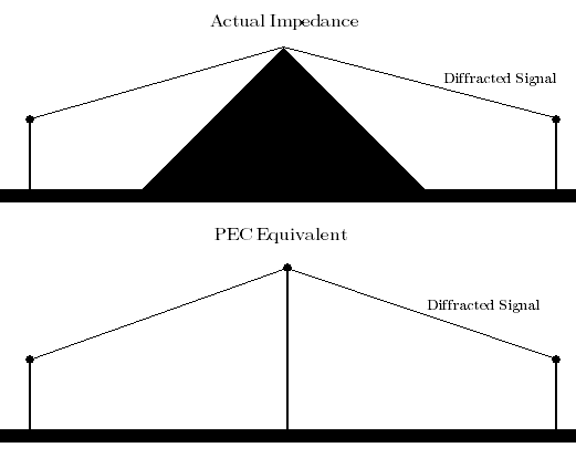
Figure 1. Terrain Modeled as Perfect
Electric Conductor
Since calculating terrain diffraction is a
mathematically intensive, Dekalb Telecom has simplified
the terrain diffraction calculations by utilizing linear
approximations to estimate terrain diffraction at most
points. Our terrain diffraction algorithm works by
calculating the wedge points, essentially terrain that
intersects the line of sight, between the sending
antenna and each one of the pixels at the edge of the
cell site map. Once the terrain diffraction was
calculated at the edge of the map, terrain diffraction
can be estimated on the interior of the map. Notice the
lines on the bottom left side of Figure 2 which shows
the interpolated terrain diffraction for cell site A.
Movie 1 demonstrates how our terrain diffraction
determines the wedge points for 90°
sweep of cell site A. Our terrain diffraction model
reduces the amount of time required to do the
diffraction calculations from approximately 640 hours to
2 hours for each map.
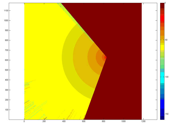
Figure 2. Terrain diffraction for cell
site
A.
Movie 1. Demonstration of linear
interpolation of terrain diffraction for cell site A.
For our case study, all of the transmitters are in the valley of Santa
Clara, California, and we’re only concerned with
matching our predictions against data collected on the
road. There are very few roads (and very few people)
high up in the mountains, so it is simplest to simply
ignore the terrain diffraction.
Since we are ignoring the terrain, our algorithm only
takes into account the clutter. It is worth noting that
only 7 of the 17 listed clutter types are actually
present in the 8 cell sites that are being analyzed:
| Present |
Not Present |
| Inland
Water |
Sea |
| Open |
Villages |
| Cropland |
Urban Open Space |
| Forest |
Residential High Vegetation |
| Parks |
Dense Urban |
|
Residential Low Vegetation |
Dense Urban High |
| Urban |
Industrial |
| |
Building Blocks |
| |
Airport |
To
measure the amount of clutter and the impact of the
clutter in the 4 sites with measured data the algorithm
iterates over the perimeter of the map. At each point on
the perimeter the algorithm calculates the
polar-coordinate ray between the map border and the
transmitter. After calculating the ray, the algorithm
starts at the transmitter and steps towards the map
border along the ray. At each grid point along the ray
path with a non-zero signal strength the algorithm
records the clutter, the distance from transmitter, and
the signal strength. The clutter is entered into the
matrix A,
which is a 17-column matrix with each column
corresponding to a clutter type. (10 of the columns end
up being all-zero.) The signal strength and the distance
from the transmitter are entered into a column vector
called b.
After the entire border has been traversed, the process
is repeated for the other 3 cell sites. (The
A and
b matrices from all of the 4 cell sites are vertically concatenated
together.) At this point the algorithm deletes the
all-zero columns of
A to prevent
the creation of a singular matrix. Once
A has been
pruned, we can finally perform the matrix algebra to
solve for x, a column vector with the clutter
coefficients:
x
= (ATA)-1 * ATb
Now the process of traversing the perimeter is repeated
to generate the actual predictions. As the algorithm
steps outwards from the transmitter towards a point on
the border the clutter coefficients are used to adjust
for the clutter along the way:
PR = PT
+ GT + GR – 20log10(r)
- 20log10(f) + 20log10(c/4π) –
a*x(1) – b*x(2) – c*x(3) - …
In
this equation, a is the number of type-1 clutter pieces
between the transmitter and the current location.
b
is the number of type-2 clutter pieces, c is the number
of type-3 clutter pieces, etc.
|