Multiple methods were applied and analyzed in the creation of the propagation model for phase 1. Section one explains the implemented model used to predict the received power strengths. Section two describes other methods that were tested and researched, and why they were not used in the final model.

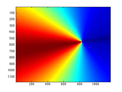
The power received at any particular location is dependent on the orientation from the transmitting antenna. Most cellular base stations have a half power bandwidth of 120 degrees. This means that the power transmitted by the antenna is halved at an orientation of 60 degrees from the antennas peak direction. In addition to half power bandwidth, most base station antennas have a front-to-back gain ratio of at least 25dB [1]. These specifications were used to create a vector of angles and a vector of expected gains. MatLab's polyfit function was used to interpolate between these vectors and create a fourth degree polynomial for the gain as a function of azimuth.

x = [0 2 20 60 120 180]; % angles in degrees
y = [1 1 0.9 0.5 0.1 0.003162277]; % linear gain
P = polyfit(x,y,4); % find a line of best fit
Results in:
P = [-5.0648e-9, 1.9784e-6,-2.1432e-4,-0.0015,1.0018]

The fourth degree polynomial response corresponding to the base stations direction and orientation is shown in Figure 1.

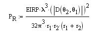
The Friis free-space link budget formula was used as a foundation for estimating the received power at a distance r from the transmitting antenna. The log form of the equation is given as:

P_R = P_T + G_T + G_R + 20log(λ) - 20log(4π) - PL

The variable PL represents path loss and includes the loss due to distance separation and also diffraction, terrain, etc. The path loss exponent model combines all these losses and attaches them as an exponent, n, to the distance loss:

PL = 10nlog₁₀(r)

The value of n is always chosen so as to minimize the mean square error between the measured path loss and the estimated path loss. This results in n being defined as:

PL_i = path loss at each measured location (obtained from Friis free-space equation)
R_i = distance at each measured location

The path loss at each given location was calculated with the power received data for Cell_Info_A through D using the link budget equation. Each path loss value was then separated into 1 of 17 groups corresponding to each measured locations environment or "clutter" value. A path loss exponent, n, was then calculated for each of the 17 different clutter groups. A table of the calculated path loss exponents is shown below.

Clutter Class	Path Loss Exponent (n)
1. Sea	2.8954
2. Inland water	2.8954
3. Open	2.8071
4. Cropland	2.7410
5. Forest	2.7119
6. Parks	2.7816
7. Villages	2.8428
8. Urban open space	2.8071
9. Res. high vegetation	2.7119
10. Res. low vegetation	2.7816
11. Dense Residential	2.7969
12. Urban	2.7838
13. Dense urban	2.8000
14. Dense urban high	2.8200
15. Industrial	2.8428
16. Building blocks	2.8428
17. Airport	2.8071

For clutter values that did not have received signal strengths, the n path loss exponent values were chosen to match a similar clutter value that did. For example, the clutter value "sea" was chosen to have the same path loss exponent as "inland water" since there were no received power levels to estimate the path loss exponent for the sea.

The estimated received signal power for maps A through D using this model are analyzed here.

The file pReceivedModel.m calculates the gain as a function of azimuth, the distance from each cell to TX, and the estimated path loss for the maps A-D. These values are all stored in matrices to act as easy look up tables. The file also calculates the N values and stores the estimated power received in the structure field variables(i).myguess.

Terrain diffraction was estimated using the Geometrical Theory of Diffraction (GTD) formula in which any obstruction is treated as a perfect electrical conducting wedge [2].

A linear (y=mx+b) function was calculated to represent a line-of-site path from the top of the transmitter to the top of the receiver. The function findpath.m was written to find and return the cell locations that fell in a straight line from the receiver to the base station. Then, storeDiffraction.m looped through each one of the cell locations in the path from the transmitter to the receiver and checked to see if the terrain blocked the line-of-sight (y=mx+b) path. If terrain blocked the line-of-sight path then storeDiffraction.m took the tallest obstruction and estimated the power received using the GTD formula.

This method was first tested with Cell_Info_A. The function was set to loop through the received power locations and determine if there was an LOS obstruction between the TX and RX. If there was, the received power was estimated according to GTD. The remaining received powers that did not contain an LOS obstruction were used to calculate a path loss exponent, n, based on the location clutter (just like Section 1). Which, if implemented correctly, should cause the path loss exponent values to be a better representation of the clutter zones. Comparing Cell_Info_A with Team1_Guess_A resulted in:

Site Cell_Info_A, mean of +3.09 dB, std dev of 7.83 dB
Average Error of (mean = 3.1 dB, sigma = 7.8 dB) for 1 site(s)
Raw Performance Score (RPS): 7.9

The diffraction and path loss exponent models combined have a lower RPS than just the path loss exponent here; however, the code took twenty minutes to run on 14,994 cells. Since the compared locations for maps E-H are unknown it means the model would have to analyze more than 1 million cells for obstruction. This would result in days of computation and thus the diffraction model was dropped.

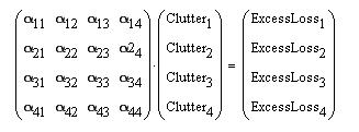
The next proposed model was to use the function findpath.m to count the number of different clutter zones the signal passes through from the transmitter to receiver. Using these values a mean square error blockage loss can be calculated for each clutter zone. This method can best be described by the following equation [3]:

PL_i = 20log₁₀(r_i) + a₁Clutter₁ + b₁Clutter₂ + ... + q₁Clutter₁₇
a₁ = Number of Clutter₁ zones between TX and RX
b₁ = Number of Clutter₂ zones between TX and RX

Or, in a simplified matrix form:

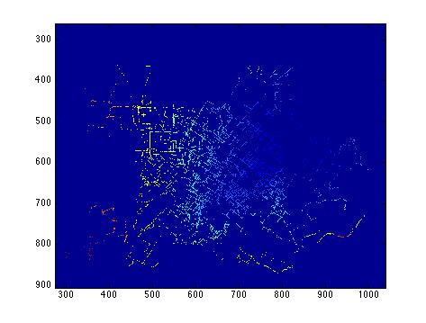
To minimize the degrees of freedom, only the four most common clutter zones between the TX and RX were used to create a blockage loss: Urban, Cropland, Parks, and Res. low vegetation. The biggest problem with this method is best shown in the following graphic:

Figure 2. Path loss as a function of clutter blockage.

The number of clutter zones measured far away from the TX is much greater than the number of clutter zones near the TX so the path loss increases. This makes intuitive sense because as a signal propagates through more blockage you expect the signal to decrease. However, this does not adequately estimate bloackage close to the TX. So, the blockage losses where then calculated based on the distance from the TX. From this point on the clutter values became more of guessing game since some matrices would be non-invertable. In addition, it was pointless to use blockage loss if the RX had a LOS path from the TX (i.e. on a hill). These discrepancies threw off the clutter values at varying distances and increased the squared error, so the model was dropped.

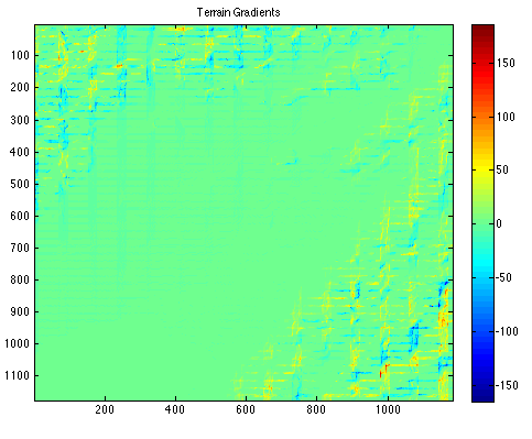
This model attempted to find diffraction and wedge points based on the areas terrain gradient. The difference of the terrain model was taken both horizontally and vertically to come up with an estimate for the total terrain change for each cell. The code that produces the gradient is shown below:

[nrows ncols] = size(Cell_Info_A.data);
horizontal_gradient = diff(Cell_Info_A.terrain);
horizontal_gradient = [zeros(1,ncols);horizontal_gradient]; % zero pad removed row
vertical_gradient = diff(Cell_Info_A.terrain'); % take difference of cols
vertical_gradient = vertical_gradient'; % transpose back
vertical_gradient = [zeros(nrows,1) vertical_gradient]; % zero pad again
total_gradient = vertical_gradient+horizontal_gradient;