
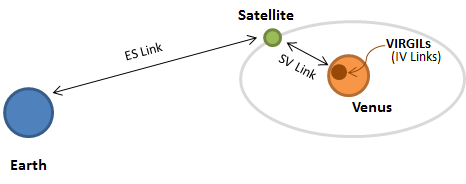
Figure 1. Mission communication links.
The mission will consist of three communication links illustrated in Figure 1. 1) Earth-to-Satellite (ES) link, 2) Satellite-to-VIRGIL (SV) link, and 3) Inter-VIRGIL (IV) links.
ES (Earth-to-Satellite) Link
For the communication between the Earth and the satellite, NASA Deep Space Network (DSN) is employed [1]. The DSN is a world-wide network of located in California, Spain and Australia. The antennas are placed 120-degree apart to allow constant observation of space crafts. The link operates at X-band, and the uplink (from Earth to the satellite) operates at 7.3 GHz containing the coded instructions and the downlink (from the satellite to Earth) operates at 8.4 GHz containing the seismic data. At the ground station, the 34-m high gain antenna is used to receive the signal from the satellite. To overcome low signal-to-noise ratio (SNR), the modulation scheme employed in our mission is BPSK (Binary phase shift keying). For the error correction, the 1/2 turbo code is employed for error correction to achieve high channel capacity. The schematics of the decoder is shown in Figure 5 [2].

Figure 2. Three 34m (110 ft.) diameter Beam Waveguide antennas at Goldstone Complex, located in the Mojave Desert in California.

Figure 3. Satellite downlink from Earth DSN antenna.

Figure 4. Satellite uplink to Earth DSN atenna.
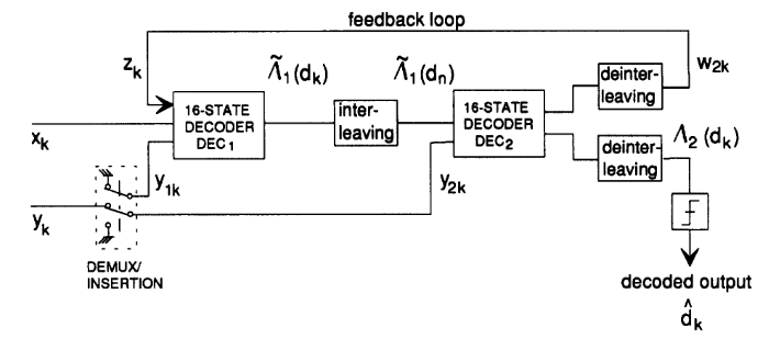
Figure 5. The FEC decoder [2].
SV (Satellite-to-VIRGILs) Link
Leveraging NASA's knowledge of the Venusian atmosphere from the Mariner 2 and Mariner 5 missions in Figure 6, choosing a wavelength of 4.1cm (roughly 7.3GHz) will give us an optimum frequency [3].
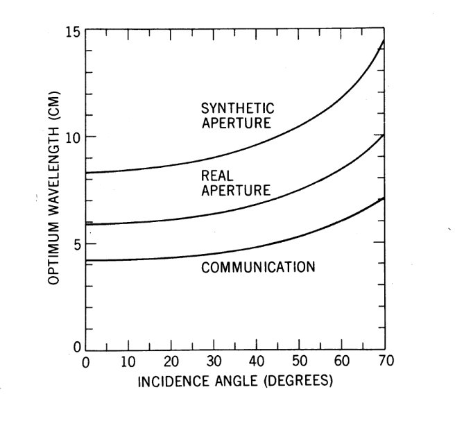
Figure 6. Optimum wavelength vs. incidence angle on the communication over the Venusian atmosphere [3].
Figures 7 and 8 detail the Downlink and Uplink, respectivly. Figure 7 shows that receiving a signal from the orbiter results in 102dB of gain. Figure 8 shows that transmitting to the orbiter gives us an astounding 277MW of EIRP, or 180.66dB of gain.
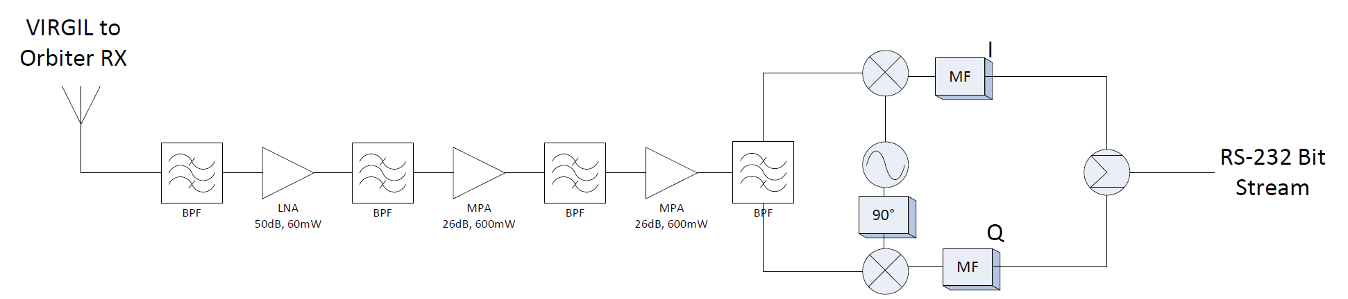
Figure 7. VIRGIL Downlink from Orbiter.
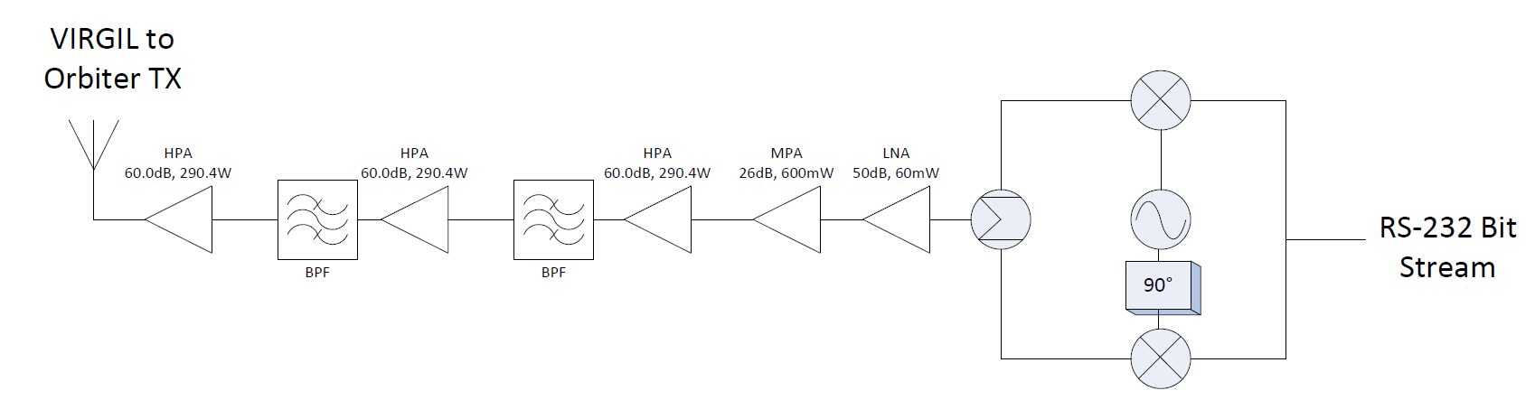
Figure 8. VIRGIL Uplink to Orbiter.
IV (inter-VIRGILs) Links
Communications between VIRGILs will be handled by in an ad-hoc way. Each VIRGIL will have a monopole antenna for communicating with other VIRGILs. Realizing that our data packets are small - each VIRGIL will only generate 3 bytes of data per seismic event - we can choose a lower frequency and have less path loss.
From Figure 9, the VIRGILs will have an estimated loss factor of 5.5. From this loss factor, we can calculate that the VIRGILs will have a path loss of roughly 5.5/λ^2 dB/km, which for our which for our 300MHz frequency works out to be 5.5dB/km [1]. The SiCLOPS mission can draw the following conclusions:
- Transmit small, easily encodable/modulated data. The less the better. SiCLOPS' processor has a RS-232 output that will be modulated using BPSK, and each data packet will be 3bytes long (24 bits), plus our CRC.
- Employ forward error correction.

Figure 9. Loss Factor Calculator including Collected Data from Mariner 5.
Using an ad-hoc network of VIRGILs allows the SiCLOPS program a few extra degrees of freedom not normally associated with planetary exploration:
- SiCLOPS can leverage fully documented, well supported, and most importantly, reliable routing algorithms to ensure that the VIRGIL in communication with the orbital satellite will always have the latest and most up-to-date activity from the VIRGILs. Dijkstra's Algorithm is the optimum choice for this, as it has the shortest path tree to a particular point. VIRGILs are most concerned with the shortest PHYSICAL distance and will be able to calculate paths to the transmitting VIRGIL based on Received Signal Strength Indicators (RSSI).
- The loss of any finite number of VIRGILs will not affect the outcome of the mission. Although possibly making a suboptimal configuration of VIRGILs, losing a VIRGIL will not be a mission failure as it would be on a single rover type mission.
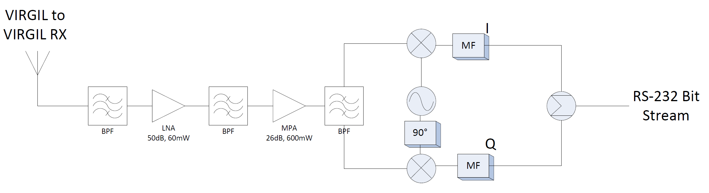
Figure 10. Receive chain of VIRGIL.

Figure 11. Transmit chain of VIRGIL.
Data Compression
Seismic data has different characteristics from the standard communicated data of video, pictures, etc. Seismic measurements are typically composed of a large amount of low frequency content, and the statistics of previously measured seismic occurrences on Earth can be leveraged to maximize the compression ratio [5,6]. The Steim 2 compression method is frequently used for seismic data compression due to its low complexity in implementation which lends itself towards use at the sensors in a distributed sensor system [7].
Steim 2 is a first difference technique where frames of data are made by giving the absolute value at the first point, and expressing the next data points as the difference between the given value and the following data points. The method expresses small differences using fewer bits than larger differences. For example, one byte is used to represent differences between -128 and +127, and two bytes are used to represent differences between -32768 and +32767. Bits in the header are used to indicate how many differences are stored in each word which allows the decoder to determine how many data points are in each word in the frame despite the variable bit length representation of data value differences. With its overhead and data frame size of 512 bits, the Steim 2's best possible compression ratio is 6.74 with the better compression ratios during periods of low seismic activity [7].
In evaluating the compression ratio for seismic data, the testing can be separated into time periods of calm and periods of seismic activity. Due to the steadiness of calm periods, the differences are smaller, and the Steim 2 compression technique is more effective. This means the compression ratio is dependent on the input data. The actual compression ratio for measured seismic data on Earth is around 2 for periods of seismic activity and 5 for calm periods [5]. The seismic data characteristics will be roughly the same on Venus, but Venus is assumed to be calmer than Earth. So, Steim 2 compression is conservatively expected to provide an average compression ratio of 4, although the sensor communication system will have to be designed to operate with a compression ratio as low as 2 for times of high seismic activity.

Figure 12. 14 hours of seismograph reading from Illinois [8] on 7/22/2014. Green indicates horizontal motion. Blue indicates vertical motion. Most seismic activity is transitory with the surrounding time filled with low difference data.
Cyclic Redundancy Check: Transmitter calculates R based on a previously determined n+1 bit G and the following equation
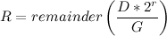
Transmitter sends the following packet

Receiver divides received [D R] by G, and an outcome of 0 indicates error free transmission [9].
We elected to handle bit errors by packet retransmission instead of forward error correction due to the limited computational ability and sufficient memory on the chosen processing systems. Cyclic redundancy check will be used for error detection since it is easily implemented in hardware which will help with the limited computational resources of the sensor. For our maximum packet length of 240000, an r of 64 was chosen as being appropriately large without introducing too many redundant bits.
[1] Deep Space Network - http://deepspace.jpl.nasa.gov/.
[2] Berrou, C.; Glavieux, A; Thitimajshima, P., "Near Shannon limit error-correcting coding and decoding: Turbo-codes. 1," Communications, 1993. ICC '93 Geneva. Technical Program, Conference Record, IEEE International Conference on , vol.2, no., pp.1064,1070 vol.2, 23-26 May 1993.
[3] K.R. Richter. "Propagation of Radio Waves Through the Lower Atmosphere of Venus." NASA Goddard Space Flight Center. Aug. 1972. Internet, http://ntrs.nasa.gov/archive/nasa/casi.ntrs.nasa.gov/19720024535.pdf
[4] Wikipedia. "Low Energy Adaptive Clustering Heirarchy." Internet: http://en.wikipedia.org/wiki/Low_Energy_Adaptive_Clustering_Hierarchy, May 1, 2014 [July 23, 2014].
[5] S. F. Newman. (Dec. 12, 2006). Seismographic Data Compression ? Appliying Modified Tunstell Coding [Online]. Available: https://www.tacoma.uw.edu/sites/default/files/global/documents/institute_tech/snewman.pdf
[6] Nijim, Y.W.; Stearns, S.D.; Mikhael, W.B., "Lossless compression of seismic signals using differentiation," Geoscience and Remote Sensing, IEEE Transactions on , vol.34, no.1, pp.52,56, Jan 1996
[7] Peterson, C.V.; Hutt, C.R., "Lossless compression of seismic data," Signals, Systems and Computers, 1992. 1992 Conference Record of The Twenty-Sixth Asilomar Conference on , vol., no., pp.712,716 vol.2, 26-28 Oct 1992
[8] ISGS Seismometer Data. Available: http://isgs.illinois.edu/isgs-seismometer
[9] Ch. 5: The Data Link Layer. Slide 5a-10. Available: http://www.cs.umd.edu/~shankar/417-F01/Slides/chapter5a-aus/sld010.htm